Subsurface turbulent mixing in the Bay of Bengal
Measurements
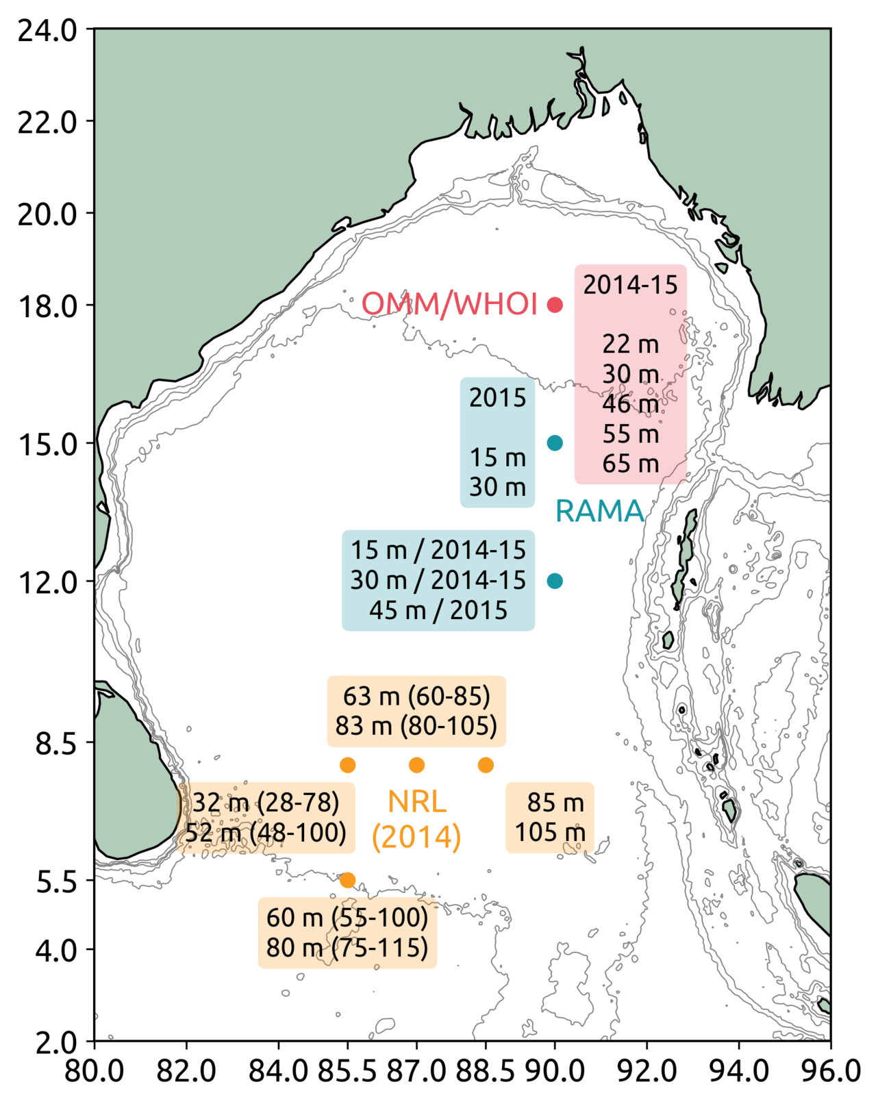
For now I am ignoring the data at 18N. The map below consists of data from RAMA moorings at 12N, 15N and the NRL EBoB array.
Specific examples
The most surprising signal is the near-molecular values observed in the thermocline (≤ 100m) at many locations in the SW Bay (off Sri Lanka).
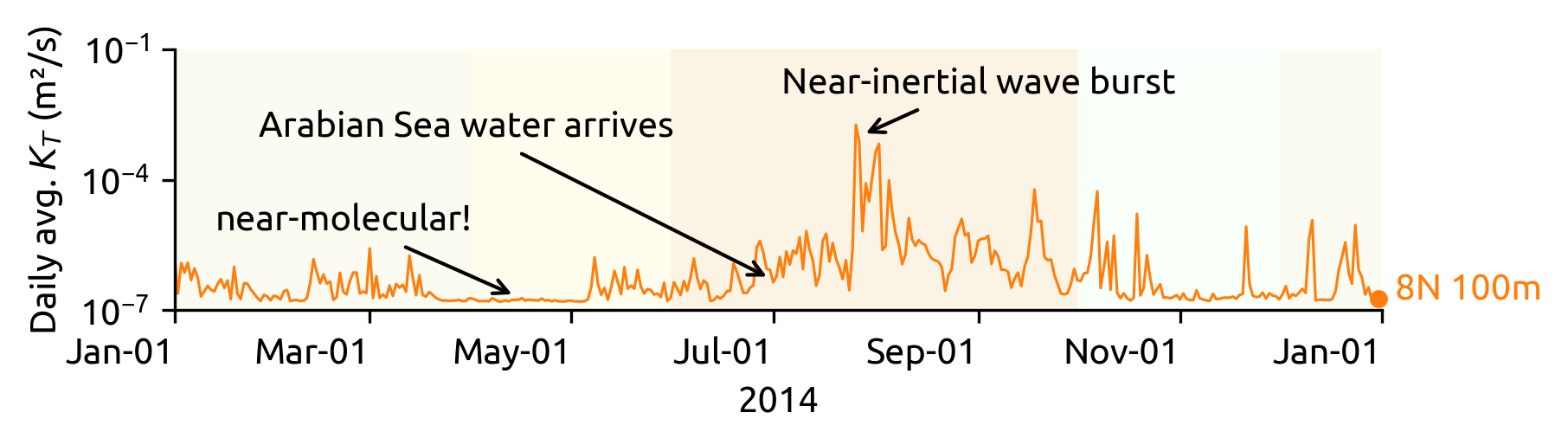
It appears that strain values are a lot smaller than expected from the Garrett-Munk spectrum.
\(K_T\) maps
Method
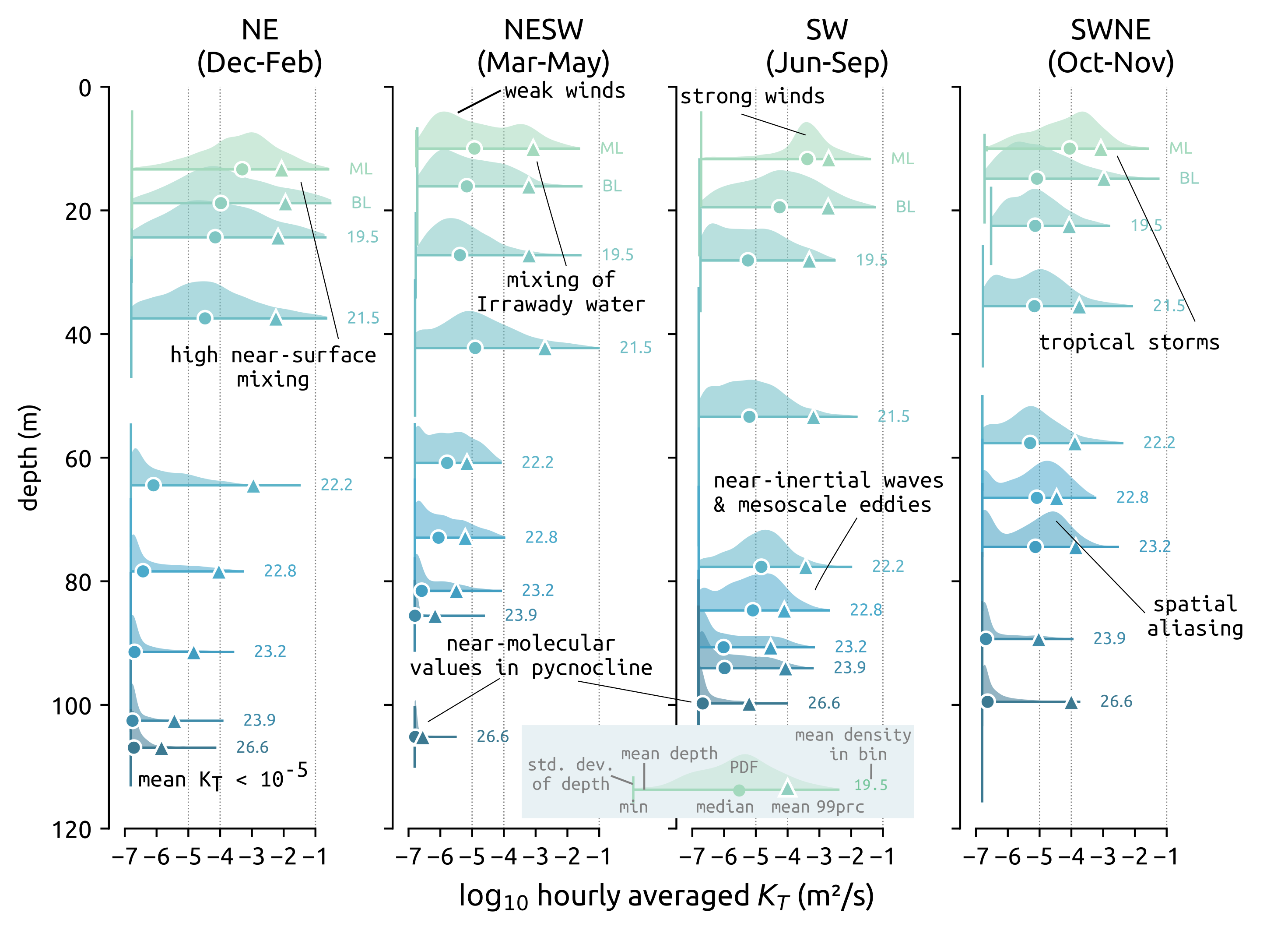
To combine data at different depths and locations throughout the Bay:
- Label each \(K_T\) estimate by whether it was made in the mixed layer ML or barrier layer BL, otherwise label it with the density of water parcel. In addition, label \(K_T\) estimate with the depth at which that estimate was made.
- Bin all observations in density space.
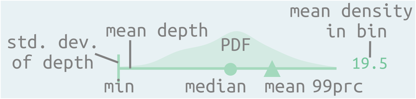
- For each density bin, estimate a "mean depth" and standard deviation of observation depths. In addition, make a kernel density estimate which is one way to estimate a PDF.
- Make a vertical profile of the PDFs:
- The baseline of each PDF is located at the "mean depth".
- The extent of the baseline ranges from the minimum value observed to the 99th percentile.
- The vertical bar at the left edge of the baseline spans one standard deviation above and below the "mean depth". This gives us an impression of how much depth space is occupied by that isopycnal bin.
- Means and medians are represented by triangles and circles respectively.
Caveats
Binning in isopycnal space results in spatial aliasing — there is no guarantee that all moorings in an isopycnal bin witness the same mesoscale/internal-wave climate. One example is the double peaked distributions in the last column of the figure below. There are 3 moorings represented in these distributions: one mooring at (85.5E, 5N) consistently shows higher mixing than the other two — (87E, 8N) and (88.5E, 8N).
\(K_T\) summary