χ-ε relations#
Motivation#
Is \(K_T = K_ρ\) at 5-m scale a good assumption in spicy regions? We make this assumption to relate \(χ_T\) (\(K_T\)) to \(ε\) (\(K_ρ\))
We have some observations of \(K_T \sim O(1) K_S\) (Nash & Moum, 2002)
\(ρ = f(T, S)\) and T, S anomalies can compensate each other, i.e. you can have \(T\) anomalies that are passive and not connected to the energy budget, so one might suspect that it’s possible to get a larger \(χ_T\) for the same \(ε\) when T-S compensation is present vs absent
From buoyancy flux#
Define \(K =χ/2/x_z^2\) \(J=-\overline{w'x'} = - K x_z\)
Start with buoyancy flux \(J_b\) which we assume to be \(Γε\) later
Signs seem right: sgn\((J_ρ) = -\)sgn\((J_T)\) and sign\((J_ρ)=\)sign\((J_S)\)
downward heat flux \(J_T < 0\) is upward density flux \(J_ρ > 0\) and upward \(J_s > 0\) is upward density flux \(J_ρ > 0\)
If \(K_T = K_S\) (e.g. Nash & Moum)
So \(K_T = K_ρ\) if \(K_ρ\) is defined so that \(J_ρ = -K_ρρ_z\)
To \(χ_ρ\)#
Gregg (1987)’s starting point is an expression for \(χ_{pe}\)
You can’t write \(χ_ρ\) using molecular gradients and diffusivity but we can make progress if we assume that \(χ_ρ = 2 K_ρ ρ_z^2\), analogous to \(χ_T\) Let’s try to derive this starting from \(J_ρ\).
So \(χ_{pe}\) is
Then,
Well, so we know now that this is all consistent
Gregg (1987) & energetics#
An alternative way to formulate the \(χ\)-\(ε\) relation is to use energetics (connected to point 2) as in Gregg (1987); Seim & Gregg (1994); Alford & Pinkel (2000). Gergg (1987)’ equation (56) is the evolution equation for \(ρ'\)
Then form an equation for perturbation potential energy \(η\)
This shows the connection between \(ε\) (\(J_b\)) and \(χ_{pe}\) (tied to \(χ_ρ\) which should be related to \(χ_T\) and \(χ_S\)).
What is \(χ_ρ\)#
Now \(χ_T\) and \(χ_S\) are “easy” to define (assuming isotropy):
where \(D_S, D_T\) are molecular diffusivities for \(S\), \(T\).
We cannot simply write \(χ_ρ = 6 \ D_ρ (∂ρ'/∂z)^2\): What is the “molecular diffusivity” of density? Instead \(χ_ρ\) must be the positive-definite dissipation term in the evolution equation of \(\overline{ρ'^2}\) derived from those for \(\overline{T'^2}\) and \(\overline{S'^2}\)
Approach of Gregg (1987)#
Gregg (1987) writes
This must assume that \(T'\) and \(S'\) are uncorrelated. As Nash & Moum (1999) show, microconductivity observations (which is a different function of \(T, S\)) can have a very different spectral shape depending on the coherence between \(T'\), \(S'\) (see below)
Assuming equililbrium energetics \(χ_{pe} = 2Γε\) (Alford & Pinkel, 2000) yields a \(ε-χ_T\) relationship, that we can then write as a \(K_T -K_ρ\) relationship
after using
For \(ε\)
Some properties:
This blows up at \(R_ρ=1 ⇒ αT_z = βS_z\) because then \(N^2 = gαT_z - gβS_z = 0\), so the gradients perfectly cancel each other. The \(ε\) equation is undefined (0/0) but I think it’s saying \(χ_T\) does not tell us anything about \(ε\) since \(T\) is totally disconnected from the energetics. This is the inverse of what I expected. But we do filter out small N2 anyway
When \(0 < R_ρ < 1\) , \(ε < 0\) but \(N^2 < 0\) so it gets filtered out.
If \(S_z = 0\), then \(K_T=K_ρ\)
What is \(R_ρ\) for NATRE? [right] Here’s the average of \(R_ρ\) along P surfaces across all profiles.
Show code cell source
import holoviews as h

hv.extension("bokeh")


Show code cell source
import hvplot.xarray
import matplotlib.pyplot as plt
import numpy as np
from datatree import DataTree

import eddydiff as ed
import xarray as xr

plt.rcParams["figure.dpi"] = 120

natre = ed.natre.read_natre(load=True)
13 40
0  values == 0
28090
/Users/dcherian/mambaforge/envs/eddydiff/lib/python3.9/site-packages/numba/np/ufunc/gufunc.py:151: RuntimeWarning: invalid value encountered in get_gradient_sign
  return self.ufunc(*args, **kwargs)
[ ] put KT/Kρ for NATRE with curve evaluated for NATRE mean Rρ
It seems like this will reduce the magnitude of the ε bump by boosting vaues above/below the bump, and reducing the bump
Show code cell source
Rρ = np.arange(-3, 3, 0.05)


def fxn_K(Rρ):
    return (1 + Rρ**2) / (1 - Rρ) ** 2


fxn_K_ideal = fxn_K(Rρ)
fxn_ε = fxn_K_ideal * (1 - 1 / Rρ)

kwargs = dict(line_width=0.75, color="k")

curve = (
    hv.Curve((Rρ, fxn_K_ideal), label="K_ρ/K_T")
    * hv.Curve((Rρ, fxn_ε), label="ε/χ")
    * (hv.VLine(1).opts(**kwargs) * hv.HLine(1).opts(**kwargs))
).opts(ylim=(0, 10), show_grid=True, xlabel="Rρ")

natre_Rρ_mean = (
    natre.Rρ.sel(pres=slice(250, None))
    .where(np.abs(natre.Rρ) < 10)
    .coarsen(pres=10, boundary="trim")
    .mean()
    .mean(["latitude", "longitude"])
    .reset_coords(drop=True)
)
natre_Rρ_mean_plot = (natre_Rρ_mean.hvplot(label="NATRE")).opts(show_grid=True) * (
    hv.HLine(0).opts(**kwargs) * hv.HLine(-2).opts(**kwargs)
)

curve + natre_Rρ_mean_plot
(
    fxn_K(natre.Rρ.sel(pres=slice(250, None)))
    .where(np.abs(natre.Rρ) < 10)
    .coarsen(pres=10, boundary="trim")
    .mean()
    .mean(["latitude", "longitude"])
    .reset_coords(drop=True)
).hvplot(label="ε_new/ε_old", ylabel="").opts(logy=True, show_grid=True)
Deriving \(χ_ρ\)#
Really really messy!
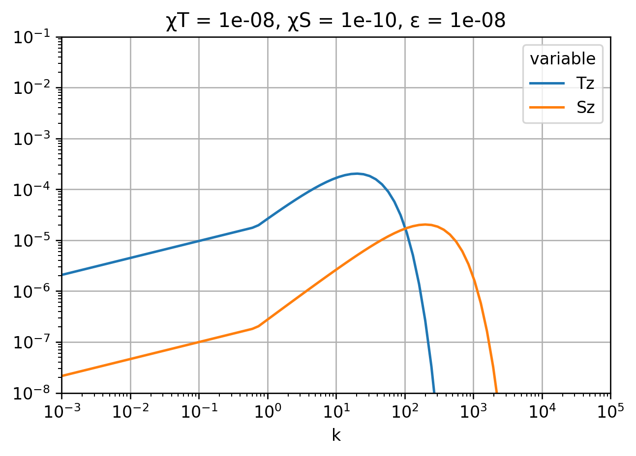
What is the spectra of \(ρ'_z\)#
Following Nash & Moum (1999)
and cospectrum can be expressed using coherence \(γ_{TzSz}(k)\) and phase \(φ(k)\)
In general if \(T_z\) and \(S_z\) are correlated then the cross-term is not negligible. Here we test this idea assuming perfect coherence amplitude, and either in-phase or 180° out-of-phase.
from dcpy.oceans import kraichnan

DT = 1.5e-7
k = np.logspace(-4, 5, 101)
# check that we recover χ
6 * DT * xr.DataArray(
    kraichnan(chi=1e-8, D=DT, eps=1e-6, nu=1e-7, k=k), dims="k", coords={"k": k}
).integrate("k").data
1.0096417568997041e-08
Show code cell source
def calculate_quantities(χT, χS, ε, N):
    from dcpy.oceans import kraichnan

    DT = 1.5e-7
    DS = 1.5e-9
    ν = 1e-6

    α = 1.7e-4
    β = 7.6e-4
    ρ0 = 1025
    Γ = 0.2
    g = -9.81

    γ = 1
    # φ = 0

    k = np.logspace(-4, 5, 101)
    kwargs = dict(k=k, eps=ε, nu=ν)
    Ψ = DataTree.from_dict(
        {
            "scalar": xr.Dataset(
                {
                    "Tz": ("k", kraichnan(**kwargs, chi=χT, D=DT)),
                    "Sz": ("k", kraichnan(**kwargs, chi=χS, D=DS)),
                },
                coords={"k": k, "χT": χT, "χS": χS, "ε": kwargs["eps"]},
            )
        }
    )

    ψ = Ψ["scalar"].ds
    Ψρ = xr.Dataset()
    Ψρ["Tz"] = (ρ0 * α) ** 2 * ψ.Tz
    Ψρ["SzTz"] = (2 * ρ0 * α * ρ0 * β * γ * np.sqrt(ψ.Tz * ψ.Sz)).real
    Ψρ["Sz"] = (ρ0 * β) ** 2 * ψ.Sz

    Ψρ["ρz"] = Ψρ["Tz"] + Ψρ["SzTz"] + Ψρ["Sz"]
    Ψρ["ρz"].attrs["long_name"] = "$Ψ_{ρz}, φ=π$"

    Ψρ["ρz_neg"] = Ψρ["Tz"] - Ψρ["SzTz"] + Ψρ["Sz"]
    Ψρ["ρz_neg"].attrs["long_name"] = "$Ψ_{ρz}, φ=0$"

    Ψ["rho"] = DataTree(Ψρ)
    Ψint = Ψ.integrate("k").reset_coords(drop=True)

    ###### Crazy assumption
    Dρ = DS

    turb = xr.Dataset()
    turb["χT"] = 6 * DT * Ψint["scalar"]["Tz"]
    turb["χS"] = 6 * DS * Ψint["scalar"]["Sz"]
    turb["χρ"] = 6 * Dρ * Ψint["rho"]["ρz"]
    turb["χρ_neg"] = 6 * Dρ * Ψint["rho"]["ρz_neg"]
    turb["χpe"] = (g / ρ0 / N) ** 2 * turb.χρ
    turb["χpe_neg"] = turb.χρ_neg

    turb["ε"] = 1 / 2 / Γ * turb.χpe
    turb["ε_neg"] = 1 / 2 / Γ * turb.χpe_neg

    Ψ["turb"] = DataTree(turb)

    return Ψ
Ψ = calculate_quantities(χT=1e-8, χS=1e-10, ε=1e-8, N=1e-2)
Ψ["scalar"].ds.to_array().plot(
    hue="variable", xscale="log", yscale="log", ylim=(1e-8, 1e-1), xlim=(1e-3, 1e5)
)
plt.grid(True)
plt.figure()
Ψ["rho"].ds.to_array().plot(
    hue="variable", xscale="log", yscale="log", ylim=(1e-8, 1e-3), xlim=(1e-3, 1e4)
)
plt.grid(True)
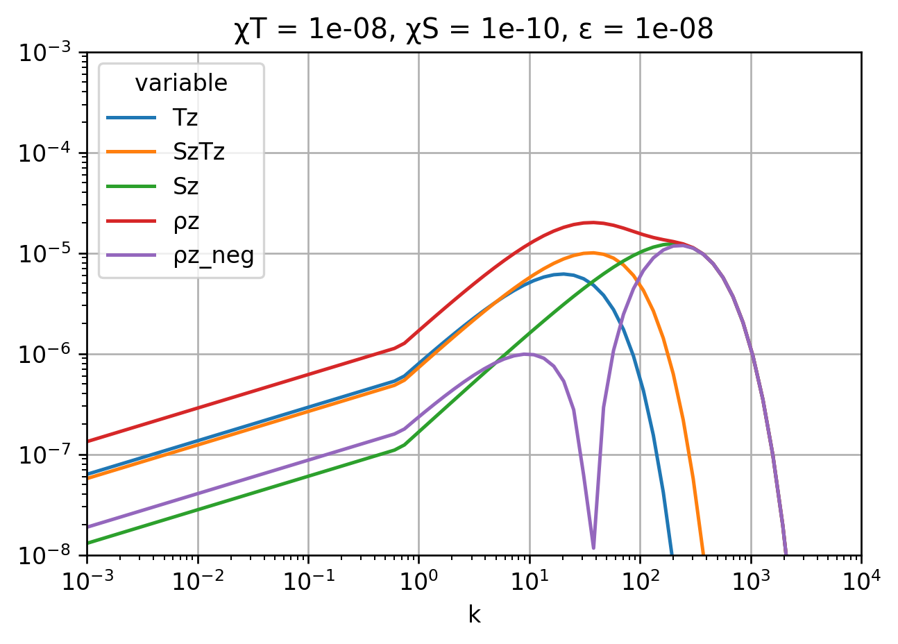
We recover \(χ_T, χ_S\). Interestingly, χpe and χpe_neg are not that different (20%) so perhaps this isn’t too bad an assumption?
display(Ψ["turb"])
display(Ψ["rho"])
<xarray.Dataset>
Dimensions:  ()
Data variables:
    χT       float64 1.007e-08
    χS       float64 1.007e-10
    χρ       float64 7.322e-11
    χρ_neg   float64 5.514e-11
    χpe      float64 6.707e-11
    χpe_neg  float64 5.514e-11
    ε        float64 1.677e-10
ε_neg float64 1.378e-10<xarray.Dataset>
Dimensions: (k: 101)
Coordinates:
* k (k) float64 0.0001 0.000123 0.0001514 ... 6.607e+04 8.128e+04 1e+05
χT float64 1e-08
χS float64 1e-10
ε float64 1e-08
Data variables:
Tz (k) float64 2.932e-08 3.141e-08 3.366e-08 3.607e-08 ... 0.0 0.0 0.0
SzTz (k) float64 2.662e-08 2.852e-08 3.056e-08 3.275e-08 ... 0.0 0.0 0.0
Sz (k) float64 6.043e-09 6.475e-09 6.938e-09 ... 1.217e-178 4.33e-219
ρz (k) float64 6.198e-08 6.641e-08 7.116e-08 ... 1.217e-178 4.33e-219
ρz_neg (k) float64 8.739e-09 9.364e-09 1.003e-08 ... 1.217e-178 4.33e-219