NATRE vs CTD-χpod#
I’m pretty sure that the CTd-χpod data needs more cleanup, but there are some interesting sampling questions explored in this notebook.
What happens if I just use single latitude or single longitude lines from the original NATRE dataset?
How do number of obs compare?
Is there some finestructure metric that tells me if we are seeing eddy stirring?
Show code cell source
%load_ext watermark
%load_ext autoreload
%autoreload 1
%matplotlib inline
import glob
import warnings
import cf_xarray as cfxr
import cf_xarray.units
import dask
import datatree
import dcpy
import distributed
import geoviews as gv
import geoviews.feature as gf
import gsw
import holoviews as hv
import hvplot.xarray
import matplotlib as mpl
import matplotlib.pyplot as plt
import numpy as np
import pint_xarray
import scipy as sp
import tqdm
import xgcm
from IPython.display import Image
from shapely.errors import ShapelyDeprecationWarning
import xarray as xr
from xarray.tests import raise_if_dask_computes
warnings.filterwarnings("ignore", category=ShapelyDeprecationWarning)
%aimport eddydiff
ed = eddydiff
xr.set_options(keep_attrs=True)
plt.rcParams["figure.dpi"] = 140
plt.rcParams["savefig.dpi"] = 200
plt.style.use("ggplot")
%watermark -iv
xr.DataArray([1.0])
The autoreload extension is already loaded. To reload it, use:
%reload_ext autoreload
/Users/dcherian/mambaforge/envs/eddydiff/lib/python3.9/site-packages/statsmodels/compat/pandas.py:65: FutureWarning: pandas.Int64Index is deprecated and will be removed from pandas in a future version. Use pandas.Index with the appropriate dtype instead.
from pandas import Int64Index as NumericIndex
geoviews : 1.9.5
xarray : 2022.6.0
dcpy : 0.2.1.dev11+gebbbf87.d20220428
holoviews : 1.14.8
xgcm : 0.6.1
scipy : 1.8.0
cf_xarray : 0.7.1.dev16+g7305fd8
hvplot : 0.7.3
pint_xarray: 0.2.1
distributed: 2022.4.0
matplotlib : 3.5.1
tqdm : 4.64.0
gsw : 3.4.0
eddydiff : 0.1
dask : 2022.4.0
numpy : 1.22.3
<xarray.DataArray (dim_0: 1)> array([1.]) Dimensions without coordinates: dim_0
Show code cell source
if "client" in locals():
client.cluster.close()
client.close()
client = distributed.Client(n_workers=6, threads_per_worker=1)
client
/Users/dcherian/mambaforge/envs/eddydiff/lib/python3.9/site-packages/distributed/node.py:177: UserWarning: Port 8787 is already in use.
Perhaps you already have a cluster running?
Hosting the HTTP server on port 61590 instead
warnings.warn(
Client
Client-70461802-5095-11ed-a6bd-3af9d394f1c6
| Connection method: Cluster object | Cluster type: distributed.LocalCluster |
| Dashboard: http://127.0.0.1:61590/status |
Cluster Info
LocalCluster
d3c44a59
| Dashboard: http://127.0.0.1:61590/status | Workers: 6 |
| Total threads: 6 | Total memory: 16.00 GiB |
| Status: running | Using processes: True |
Scheduler Info
Scheduler
Scheduler-e94c491f-83df-47b6-8785-f3f33d668e3f
| Comm: tcp://127.0.0.1:61591 | Workers: 6 |
| Dashboard: http://127.0.0.1:61590/status | Total threads: 6 |
| Started: Just now | Total memory: 16.00 GiB |
Workers
Worker: 0
| Comm: tcp://127.0.0.1:61621 | Total threads: 1 |
| Dashboard: http://127.0.0.1:61626/status | Memory: 2.67 GiB |
| Nanny: tcp://127.0.0.1:61597 | |
| Local directory: /Users/dcherian/work/eddydiff/notebooks/dask-worker-space/worker-5o5_x_fw | |
Worker: 1
| Comm: tcp://127.0.0.1:61612 | Total threads: 1 |
| Dashboard: http://127.0.0.1:61617/status | Memory: 2.67 GiB |
| Nanny: tcp://127.0.0.1:61595 | |
| Local directory: /Users/dcherian/work/eddydiff/notebooks/dask-worker-space/worker-stmte294 | |
Worker: 2
| Comm: tcp://127.0.0.1:61614 | Total threads: 1 |
| Dashboard: http://127.0.0.1:61620/status | Memory: 2.67 GiB |
| Nanny: tcp://127.0.0.1:61599 | |
| Local directory: /Users/dcherian/work/eddydiff/notebooks/dask-worker-space/worker-qv754dvy | |
Worker: 3
| Comm: tcp://127.0.0.1:61613 | Total threads: 1 |
| Dashboard: http://127.0.0.1:61615/status | Memory: 2.67 GiB |
| Nanny: tcp://127.0.0.1:61594 | |
| Local directory: /Users/dcherian/work/eddydiff/notebooks/dask-worker-space/worker-48ix56e0 | |
Worker: 4
| Comm: tcp://127.0.0.1:61625 | Total threads: 1 |
| Dashboard: http://127.0.0.1:61627/status | Memory: 2.67 GiB |
| Nanny: tcp://127.0.0.1:61596 | |
| Local directory: /Users/dcherian/work/eddydiff/notebooks/dask-worker-space/worker-erkh1o_k | |
Worker: 5
| Comm: tcp://127.0.0.1:61616 | Total threads: 1 |
| Dashboard: http://127.0.0.1:61623/status | Memory: 2.67 GiB |
| Nanny: tcp://127.0.0.1:61598 | |
| Local directory: /Users/dcherian/work/eddydiff/notebooks/dask-worker-space/worker-nqgo9r1j | |
Read datasets#
%autoreload
natre = ed.natre.read_natre(load=True)
bins = ed.sections.choose_bins(natre.gamma_n, depth_range=np.arange(150, 2001, 100))
13 40
/Users/dcherian/mambaforge/envs/eddydiff/lib/python3.9/site-packages/numba/np/ufunc/gufunc.py:151: RuntimeWarning: invalid value encountered in get_gradient_sign
return self.ufunc(*args, **kwargs)
0 values == 0
28090
natre_2m = natre.coarsen(pres=4, boundary="trim").mean()
natre_2m
<xarray.Dataset>
Dimensions: (latitude: 10, longitude: 10, pres: 995)
Coordinates:
* latitude (latitude) float64 27.5 27.1 26.7 26.3 ... 25.1 24.7 24.3 23.9
* longitude (longitude) float64 -30.7 -30.3 -29.8 -29.4 ... -27.6 -27.2 -26.8
* pres (pres) float64 10.75 12.75 14.75 ... 1.997e+03 1.999e+03
time (latitude, longitude) datetime64[ns] 1992-03-28T15:28:59.99999...
depth (latitude, longitude, pres) float64 nan nan ... 1.977e+03
Data variables: (12/23)
chi (latitude, longitude, pres) float64 nan nan ... 1.346e-10
eps (latitude, longitude, pres) float64 nan nan ... 1.079e-10
salt (latitude, longitude, pres) float64 nan nan nan ... 35.05 35.05
temp (latitude, longitude, pres) float64 nan nan nan ... 3.934 3.932
gamma_n (latitude, longitude, pres) float64 nan nan nan ... 27.98 27.98
SA (latitude, longitude, pres) float64 nan nan nan ... 35.22 35.22
... ...
Kt (latitude, longitude, pres) float64 nan nan ... 2.349e-05
KtTz (latitude, longitude, pres) float64 nan nan ... -2.118e-08
Tz~ (latitude, longitude, pres) float64 nan nan nan ... nan nan nan
chi~ (latitude, longitude, pres) float64 nan nan nan ... nan nan nan
Kt~ (latitude, longitude, pres) float64 nan nan nan ... nan nan nan
KtTz~ (latitude, longitude, pres) float64 nan nan nan ... nan nan nan
Attributes: (12/13)
Conventions: CF-1.6
netcdf_version: 4
project: North Atlantic Tracer Release Experiment (NATRE)
expocode: 32OC250_4
cast_number: 3.0
title: Microstructure profiler data from the ship Oceanus...
... ...
latitude: 27.533166666666666
longitude: -30.723333333333333
chief_scientist: Raymond W. Schmitt
data_originator: Polzin
institution: WHOI
data_assembly_center: CCHDOnatre_binned = xr.load_dataset("../datasets/natre-density-binned.nc")
natre_binned.attrs["title"] = "NATRE"
latlines = xr.load_dataset("../datasets/natre-along-lat-lines.nc")
lonlines = xr.load_dataset("../datasets/natre-along-lon-lines.nc")
section = "A05"
expocode = "74EQ20151206"
redo_finescale = False
station_bin_edges = [0, 28, 60, 82, 105, 130, 145]
filenames = ed.sections.get_filenames("A05_2015")
a05 = datatree.open_datatree(filenames["merged"])
# a05_binned = xr.load_dataset("../datasets/ctd-A05-density-binned-no-cast-131.nc").query(
# {"gamma_n": "pres < 2000"}
# )
# a05_binned_old = xr.load_dataset("../datasets/ctd-A05-density-binned.nc").query(
# {"gamma_n": "pres < 2000"}
# )
a05_binned = xr.load_dataset("../datasets/A05-2015.nc")
a05_binned.attrs["title"] = "A05"
cole = ed.read_cole()
%autoreload
ed.sections.add_ctd_ancillary_variables(a05["ctd"].ds)
ed.sections.add_turbulence_ancillary_variables(a05["chipod"].ds)
a05["chipod"].ds["Tu"] = a05["ctd"].ds["Tu"]
/Users/dcherian/work/python/cf-xarray/cf_xarray/accessor.py:1638: UserWarning: Variables {'ctd_salinity_qc'} not found in object but are referred to in the CF attributes.
warnings.warn(
/Users/dcherian/work/python/cf-xarray/cf_xarray/accessor.py:1638: UserWarning: Variables {'ctd_temperature_qc'} not found in object but are referred to in the CF attributes.
warnings.warn(
[0.02666667]
[0.02666667]
[0.08]
[0.08]
[0.02666667]
[0.02666667]
[0.02666667]
NATRE \(ε\) vs \(ε_χ\)#
fRρ = (1 - 2 / natre_.Rρ + 1 / natre_.Rρ**2).where(np.abs(natre_.Rρ) > 1)
α = gsw_xarray.alpha(natre_.SA, natre_.CT, natre_.pres)
fN = (-9.81 * α * natre_.Tz / natre_.N2) ** 2
with plt.rc_context({"lines.linewidth": 0.75}):
natre_.eps.mean("cast").cf.plot(xscale="log", color="k")
natre_.eps_chi.mean("cast").cf.plot(xscale="log")
(fN * natre_.eps_chi * fRρ).mean("cast").cf.plot(xscale="log")
Turner angle / Rρ diagnostics#
TODO#
[x] Issues with dTdz for Γ? How do I reproduce Aurelie’s dThdz?
100m fitler
Ashin uses 8m
[x] Do histogram of Rρ, Γ with depth
[ ] What is the outlier ε for A05, Rρ ~ 4
Calculation of Tu / Rρ#
Ashin et al (2022):
To estimate〈∂T/∂z, a 10s(∼8 m) low-pass filter was applied to the temperature profiles to remove high-frequency variations, and then the temperature gradients less than the accuracy of the temperature sensor (0.018°C/m) were removed.
St Laurent & Schmitt (1999):
Finestructure gradient quantities, particularly Rr and Ri, will be used extensively in the analysis that follows. To estimate the vertical gradients of scalars, we have used the slope of a linear fit over a 5-m segment, centered at each 0.5-m interval. The 5-m scale was chosen as a suitable trade-off between the need for high vertical resolution and statistically reasonable regression estimation. The magnitudes of all 5-m scalar gradients were compared to their associated standard error. Gradient quantities with standard errors larger than twice their magnitude were excluded from the analysis. … “The gradients were calculated using a 5-m scale, smoothed using a 50-m running average.”
GO-SHIP CTD-χpod
bin to 5m, difference, then run 100m smoother
Read#
Show code cell source
%autoreload
natre = ed.natre.read_natre(load=True)
natre_ = (
natre.stack({"cast": ["latitude", "longitude"]})
.drop_vars("cast")
.sel(pres=slice(250, 2000))
)
a05ctd = (
xr.load_dataset(filenames["ctd"])
.pipe(dcpy.oceans.preprocess_cchdo_cf_netcdf)
.drop_vars(["ctd_salinity_qc", "ctd_temperature_qc", "ctd_oxygen_qc", "ctd_oxygen"])
.sel(station=slice(108, 130), pressure=slice(250, 2000))
)
ed.sections.add_ctd_ancillary_variables(a05ctd)
a05_ = (
a05["chipod"]
.sel(
cleaner="none",
direction="dn",
station=slice(108, 130),
pressure=slice(250, 2000),
)
.ds
) # .ds.Tu.plot.hist()
13 40
/Users/dcherian/mambaforge/envs/eddydiff/lib/python3.9/site-packages/numba/np/ufunc/gufunc.py:151: RuntimeWarning: invalid value encountered in get_gradient_sign
return self.ufunc(*args, **kwargs)
0 values == 0
28090
/var/folders/yp/rzgd0f7n5zbcbf5dg73sfb8ntv3xxm/T/ipykernel_75453/1555697229.py:5: DeprecationWarning: Deleting a single level of a MultiIndex is deprecated. Previously, this deleted all levels of a MultiIndex. Please also drop the following variables: {'latitude', 'longitude'} to avoid an error in the future.
natre.stack({"cast": ["latitude", "longitude"]})
/Users/dcherian/work/python/cf-xarray/cf_xarray/accessor.py:1638: UserWarning: Variables {'ctd_salinity_qc'} not found in object but are referred to in the CF attributes.
warnings.warn(
/Users/dcherian/work/python/cf-xarray/cf_xarray/accessor.py:1638: UserWarning: Variables {'ctd_temperature_qc'} not found in object but are referred to in the CF attributes.
warnings.warn(
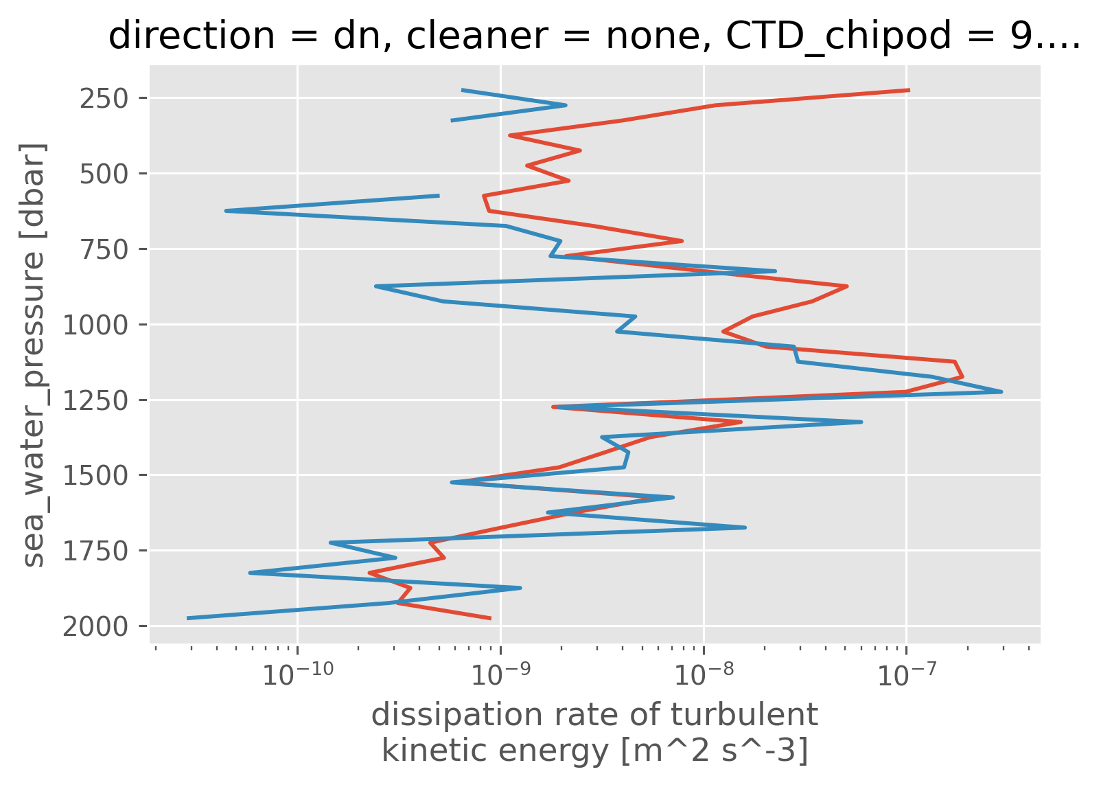
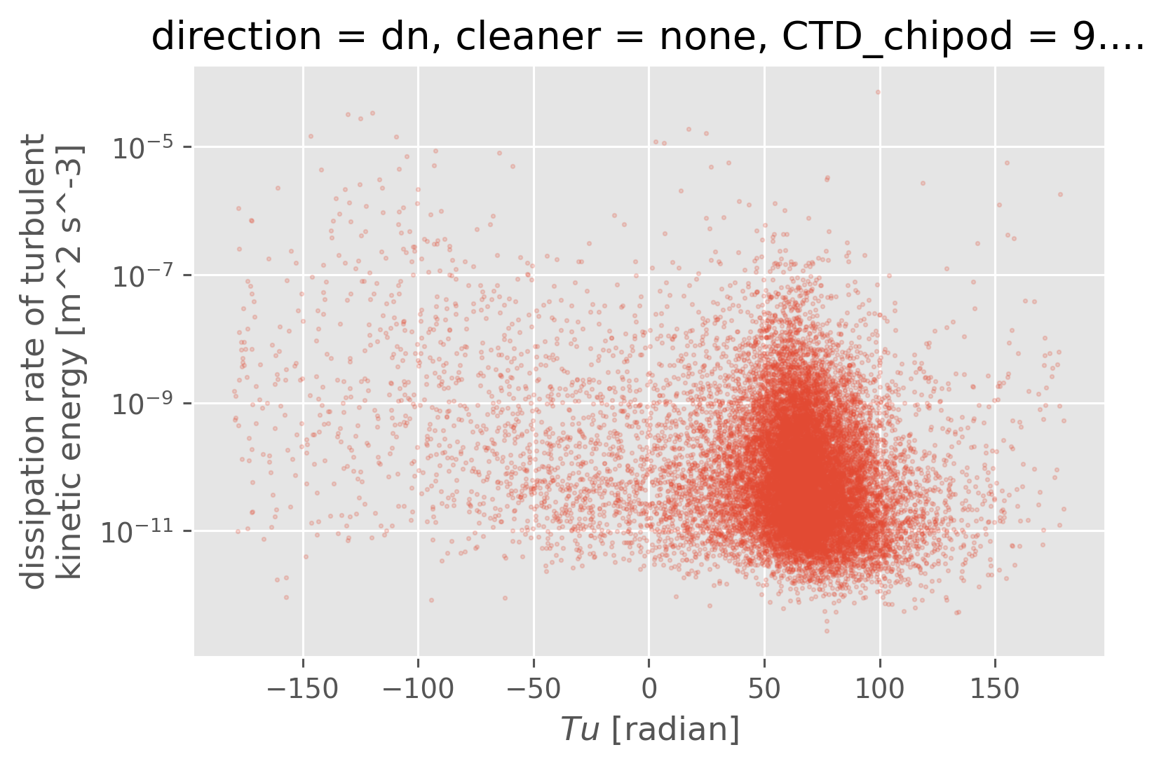
Diagnostics#
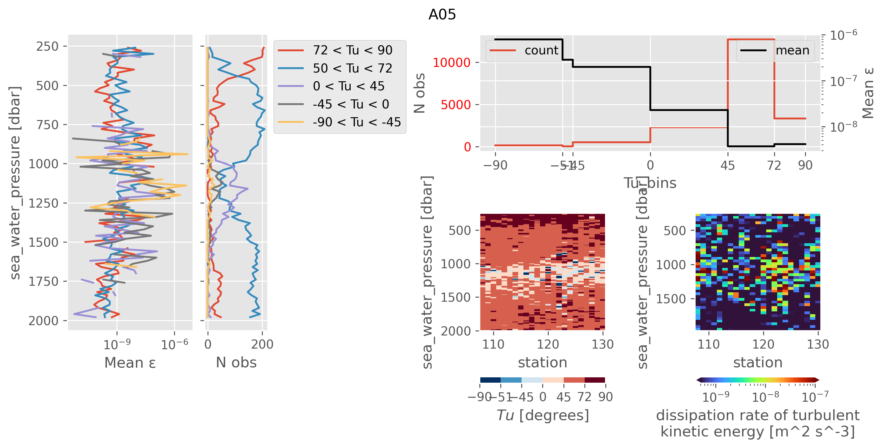
My takeaways are:
A05 sampled ocean conditions similar to NATRE in terms of Rρ.
We could throw out the small number of diffusive convection points that have really high ε (-90 < Tu < -45). This would not reduce the average ε (see next)
In the doubly stable shear turbulence regime at 1000dbar (-45 < Tu < 45) we still have high ε ~ 1e-7-ish; NATRE has 1e-10
St-Laurent & Schmitt:
Data in the density ratio range between -1 and 0 were held from the analysis, as these data are characterized by weak thermal stratification where \(θ_z\) → 0, making \(Γ\) singular.
%autoreload
ed.plot.plot_Tu_relationships(a05_, title="A05")
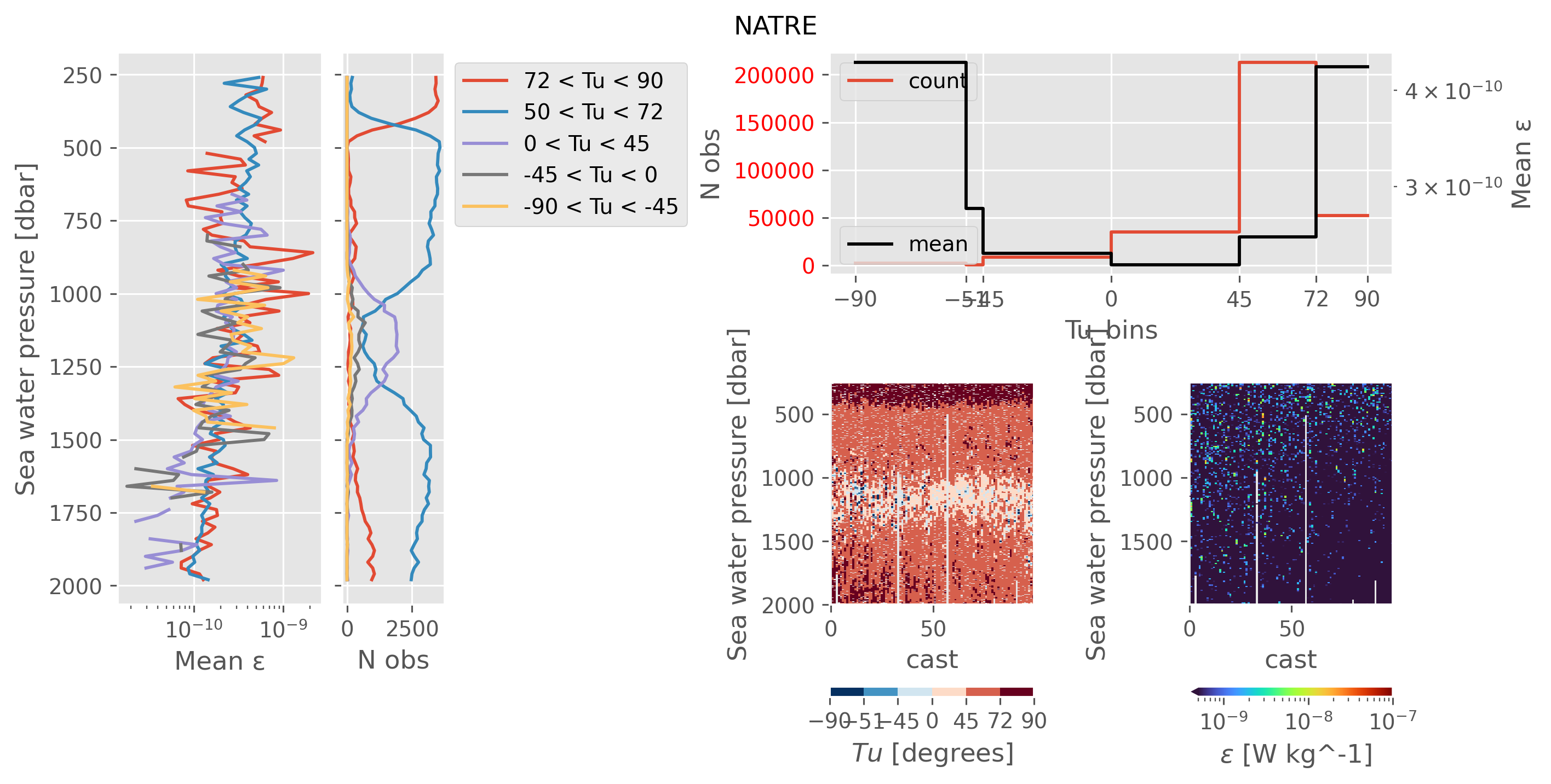
ed.plot.plot_Tu_relationships(natre_, title="NATRE")
2022-10-21 12:24:50,897 - distributed.utils_perf - WARNING - full garbage collections took 13% CPU time recently (threshold: 10%)
plt.rcParams["figure.dpi"] = 140
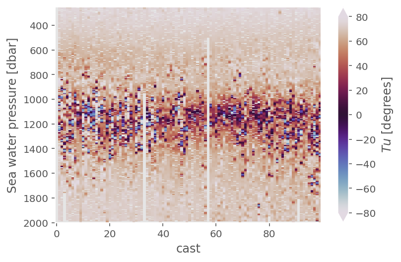
natre_.Tu.cf.plot(y="pres", x="cast", cmap=mpl.cm.twilight, vmin=-80, vmax=80)
plt.figure()
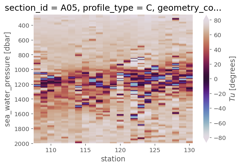
a05ctd.Tu.cf.plot(x="profile_id", cmap=mpl.cm.twilight, levels=[45, 90])
<matplotlib.collections.QuadMesh at 0x17f2c3e50>
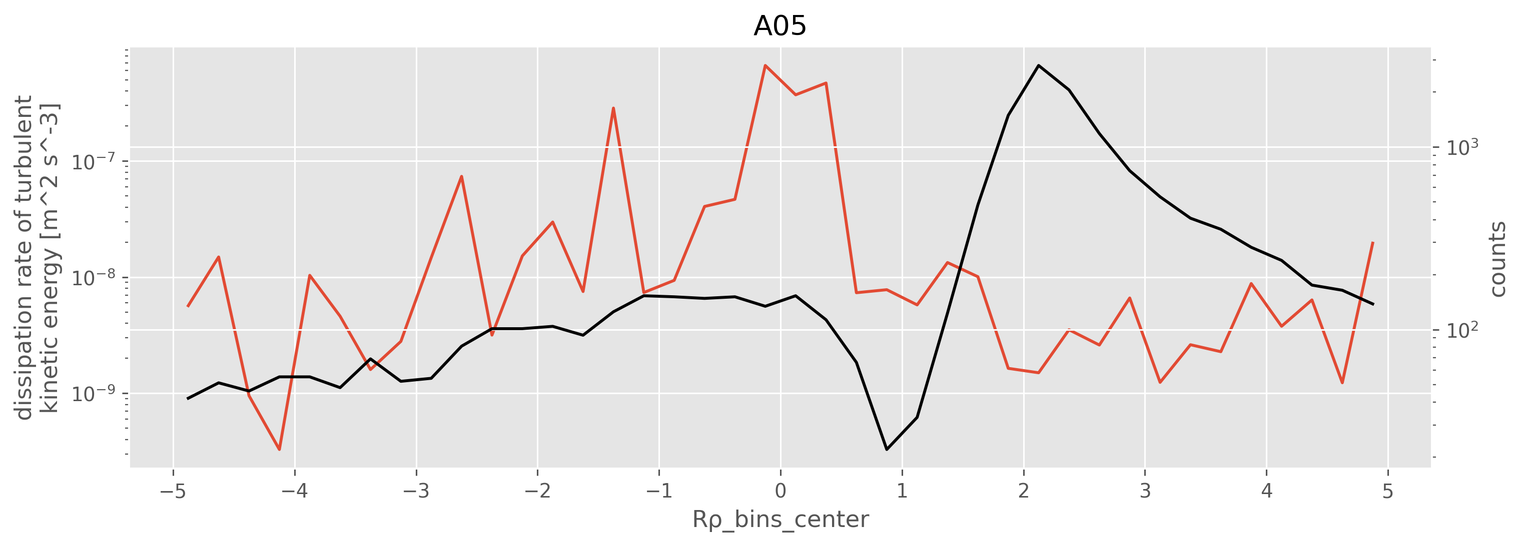
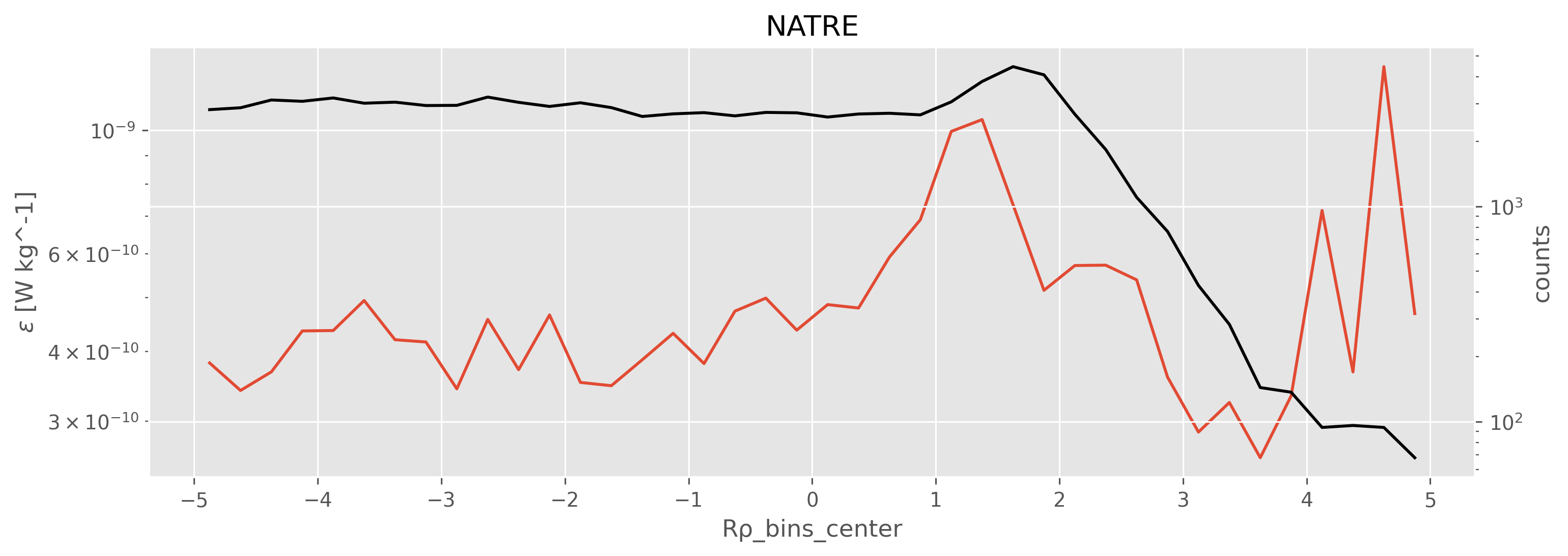
ε-Rρ#
Mean eps is high for Rρ ~ 0, compared to Rρ < 0
There are equal number of points at Rρ~0 and \(R_ρ \approx -1\)
def plot_Rrho_dependencies(eps, Rρ, title=None):
gb = eps.groupby_bins(Rρ, bins=np.arange(-5, 5.1, 0.25))
gb.mean().plot.line(yscale="log")
ax = plt.gca()
counts = gb.count().rename("counts")
counts.attrs.clear()
ax2 = plt.gca().twinx()
counts.plot.line(yscale="log", ax=ax2, color="k")
ax.set_xticks(gb._bins[::4])
ax.set_title(title)
ax2.set_title("")
plt.gcf().set_size_inches(mpl.figure.figaspect(1 / 3))
eps = (
a05["chipod"]
.ds["eps"]
.sel(
cleaner="none",
direction="dn",
station=slice(108, 130),
pressure=slice(500, 2000),
)
)
Rρ = (
a05["ctd"]
.ds["Rρ"]
.sel(station=slice(108, 130), pressure=slice(500, 2000))
.clip(-10, 10)
)
plot_Rrho_dependencies(eps, Rρ, title="A05")
plt.figure()
sub = natre.sel(pres=slice(500, 2000))
plot_Rrho_dependencies(natre.eps, natre.Rρ, title="NATRE")
pod = a05["chipod"].ds.sel(
cleaner="none",
direction="dn",
station=slice(108, 130),
pressure=slice(200, 2000),
)
pod.eps.coarsen(pressure=25).mean().mean("station").cf.plot(xscale="log")
pod.eps.where(pod.Rρ < -0.5).coarsen(pressure=25).mean().mean("station").cf.plot(
xscale="log"
)
[<matplotlib.lines.Line2D at 0x18c7608e0>]
pod["Tu"] = pod.Tu.copy(data=np.rad2deg(pod.Tu.data))
pod.plot.scatter("Tu", "eps", alpha=0.2, s=2)
plt.gca().set_yscale("log")
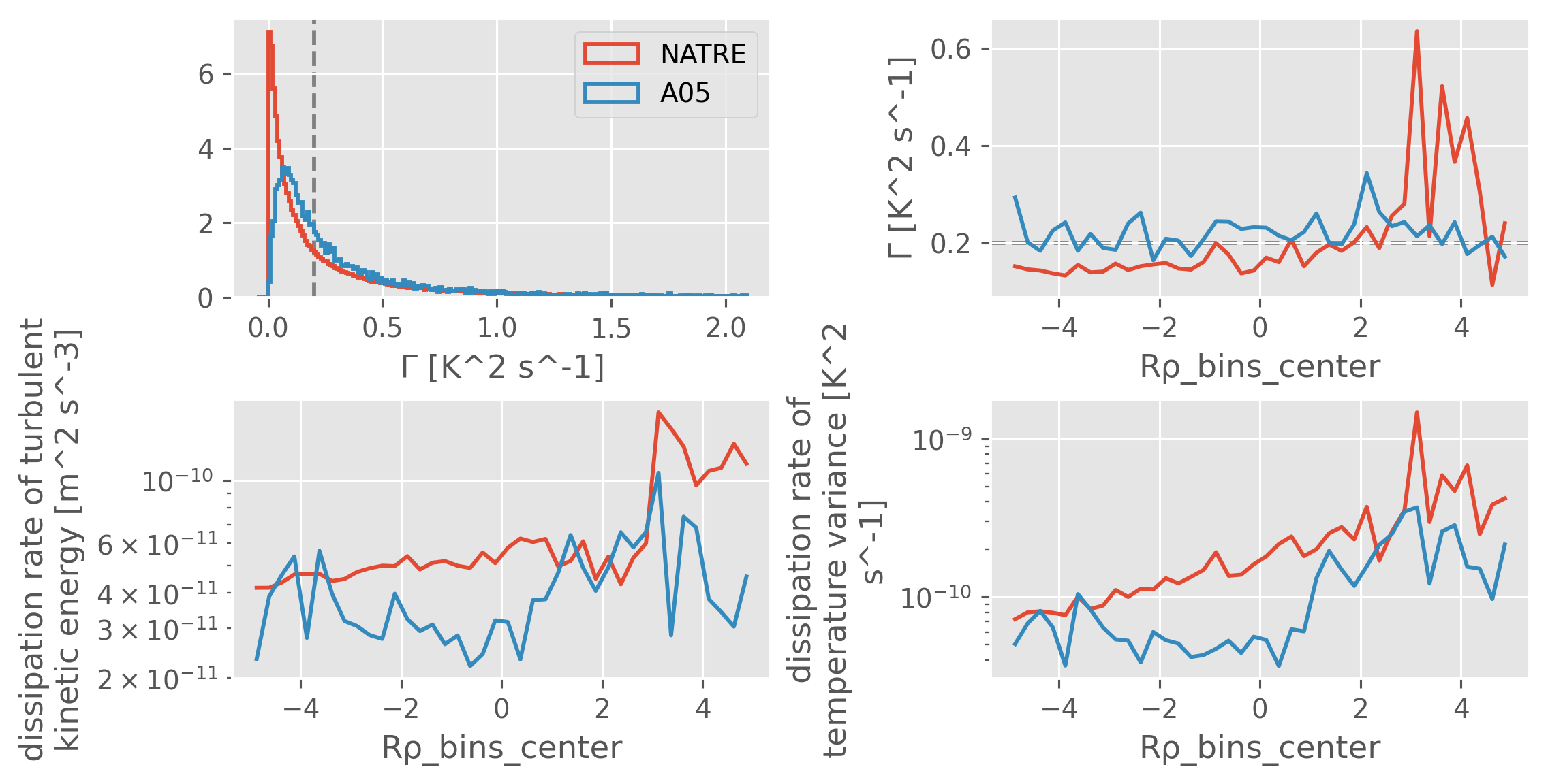
def plot_Gamma_diagnostics(datasets):
f, ax = plt.subplots(2, 2, constrained_layout=True)
for name, data in datasets.items():
data.Gamma.plot.hist(
density=True,
bins=np.arange(-0.05, 2.1, 0.01),
histtype="step",
ax=ax[0, 0],
label=name,
lw=1.5,
)
for axx, var, yscale in zip(
ax.ravel()[1:], ["Gamma", "eps", "chi"], ["linear", "log", "log"]
):
mean = (
data[var].groupby_bins(data.Rρ, bins=np.arange(-5, 5.1, 0.25)).median()
)
assert mean.ndim == 1
# display(mean)
mean.plot(ax=axx, yscale=yscale)
dcpy.plots.linex(0.2, ax=ax[0, 0])
dcpy.plots.liney(0.2, ax=ax[0, 1])
ax[0, 0].legend()
[axx.set_title("") for axx in ax.ravel()]
plt.gcf().set_size_inches(mpl.figure.figaspect(1 / 2))
data = a05["chipod"].ds
# a05["chipod"].ds["Gamma"] = (data.chi * data.N2)/(2 * data.eps * data.dThdz**2).where((np.abs(data.dThdz) > 3e-4) & (data.N2 > 1e-6))
plot_Gamma_diagnostics(
{
"NATRE": natre.sel(pres=slice(600, 2000)),
"A05": a05["chipod"].ds.sel(
cleaner="none",
direction="dn",
station=slice(108, 130),
pressure=slice(600, 2000),
),
}
)
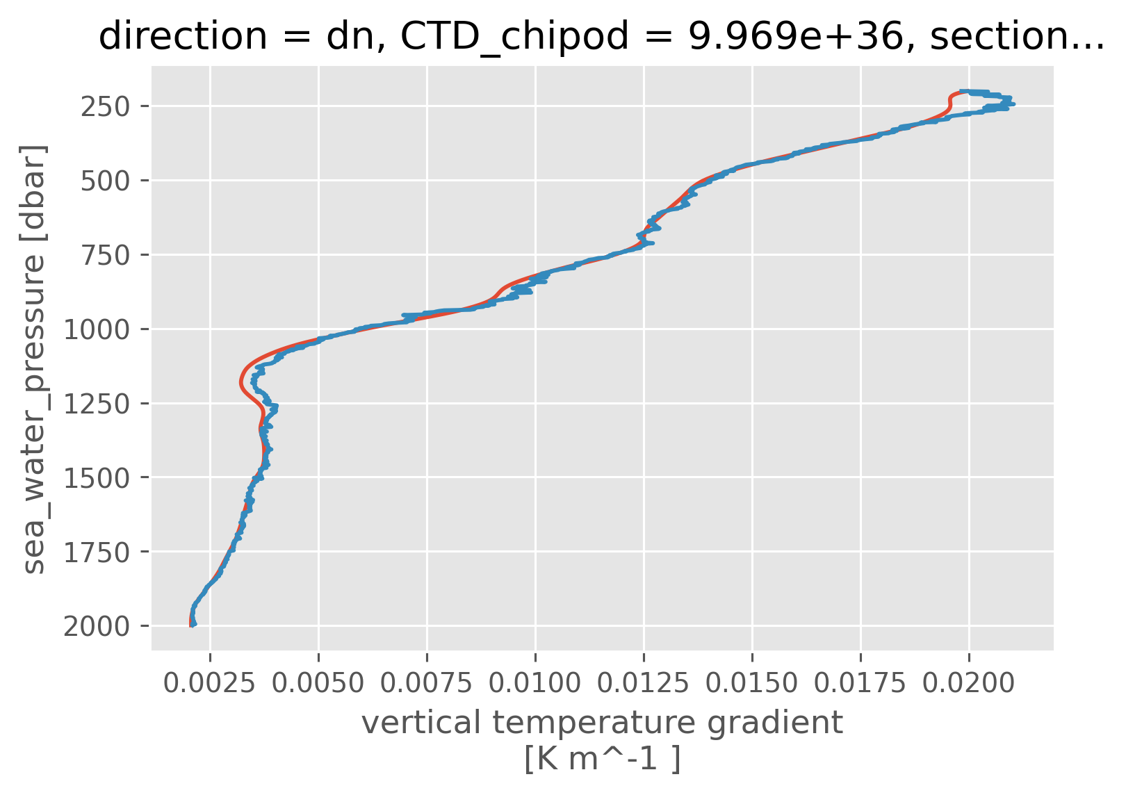
Tz vs dThdz#
subset = a05.sel(station=slice(108, 130), pressure=slice(200, 2000))
subset["ctd"].ds.Tz.mean("station").cf.plot()
subset["chipod"].ds.dThdz.mean("station").sel(direction="dn").cf.plot()
[<matplotlib.lines.Line2D at 0x1823729d0>]
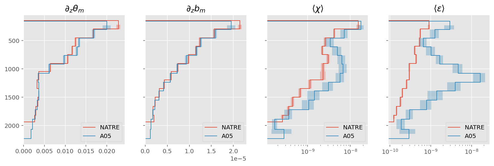
Compare to each other#
ed.plot.compare_section_estimates([natre_binned, a05_binned])
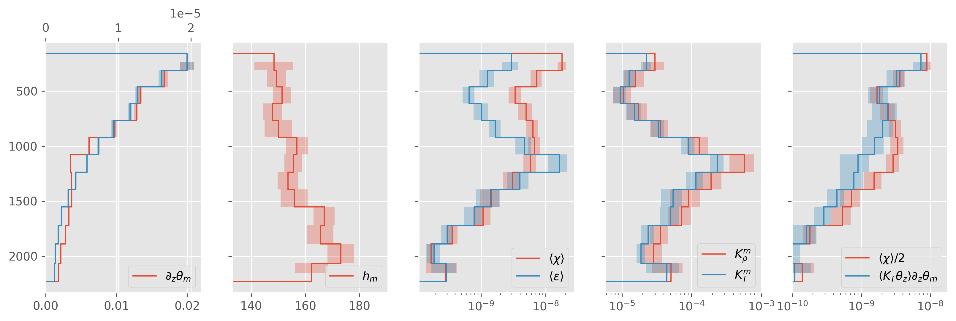
Compare individual binned residuals#
ed.plot.debug_section_estimate(natre_binned, KρTz2=True)
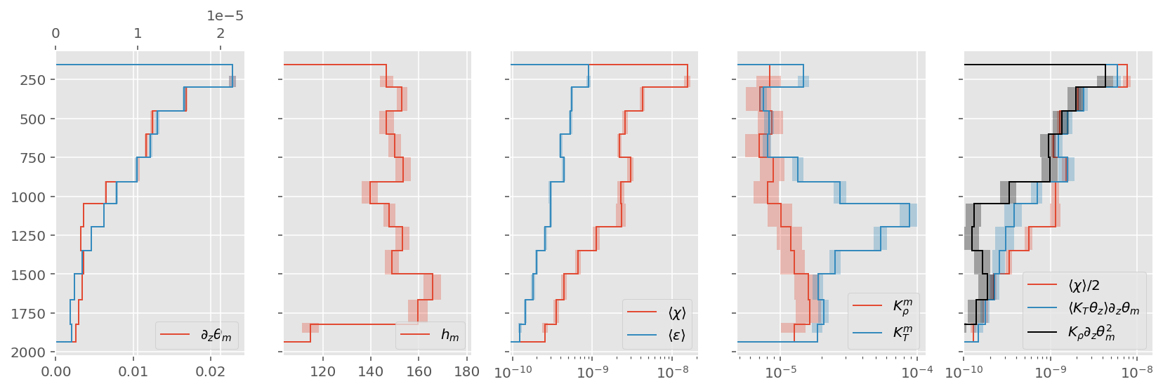
ed.plot.debug_section_estimate(a05_binned)
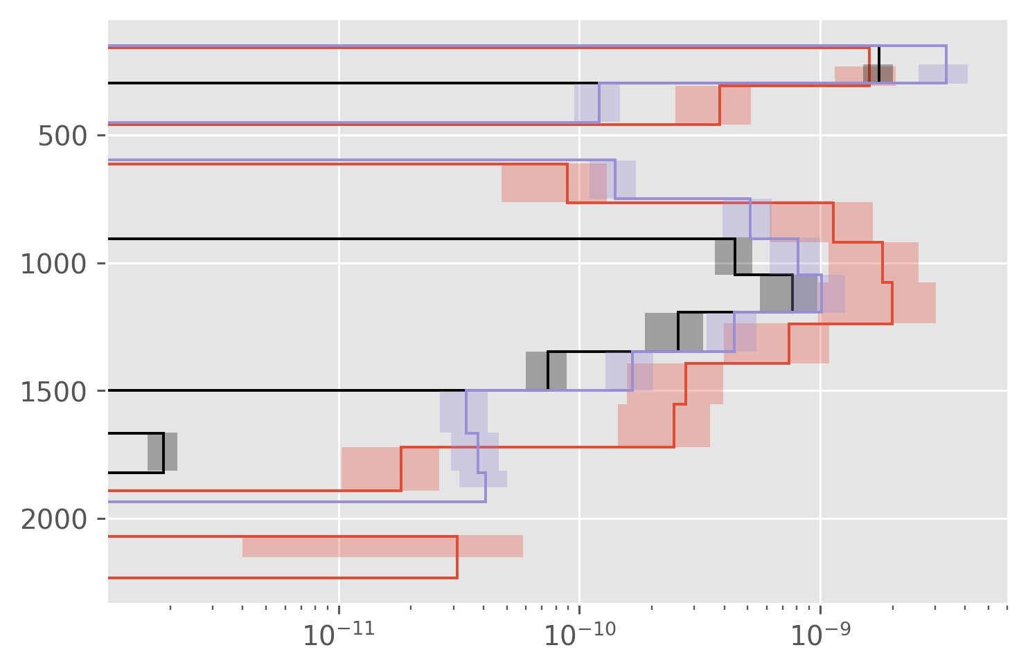
dcpy.plots.fill_between_bounds(a05_binned, "residual_chi", y="pres")
dcpy.plots.fill_between_bounds(natre_binned, "residual_chi", y="pres", color="k")
dcpy.plots.fill_between_bounds(natre_binned, "residual", y="pres", color="C2")
plt.xscale("log")
Map : Did A05 sample the “right” place?#
Locate entire cruise on map with NATRE & \(|∇^ρS|\) (averaged over 750m-1250m)
\(|∇^ρS|\) along 25°N shows a mid-depth maximum as expected (A05 latitude is approximately 24.7°N)
(
cole.salinity_gradient.sel(lon=slice(360 - 100, 345))
.sel(lat=24.7, method="nearest")
.cf.plot(robust=True, size=5, aspect=3)
)
<matplotlib.collections.QuadMesh at 0x109d17c70>
chipod = a05["chipod"].ds
with_chi = chipod.cf[["latitude", "longitude"]].where(
chipod.chi.count("pressure") > 0 # , drop=True
)
lats, lons = np.meshgrid(natre.latitude, natre.longitude)
dS = (
cole.salinity_gradient.sel(
lon=slice(360 - 80, 360), lat=slice(10, 40), pres=slice(750, 1250)
)
.mean("pres")
.hvplot(geo=True)
)
natre_casts = gv.Points((lons.ravel(), lats.ravel()))
allcasts = gv.Points((chipod.cf["longitude"], chipod.cf["latitude"]))
chicasts = gv.Points((with_chi.cf["longitude"], with_chi.cf["latitude"]))
a05_casts = allcasts.opts(size=6, color="cyan") * chicasts.opts(color="k")
(
# dS.opts(cmap="bmy")
natre_casts.opts(color="k")
* a05_casts
* gf.coastline.opts(line_width=2)
)
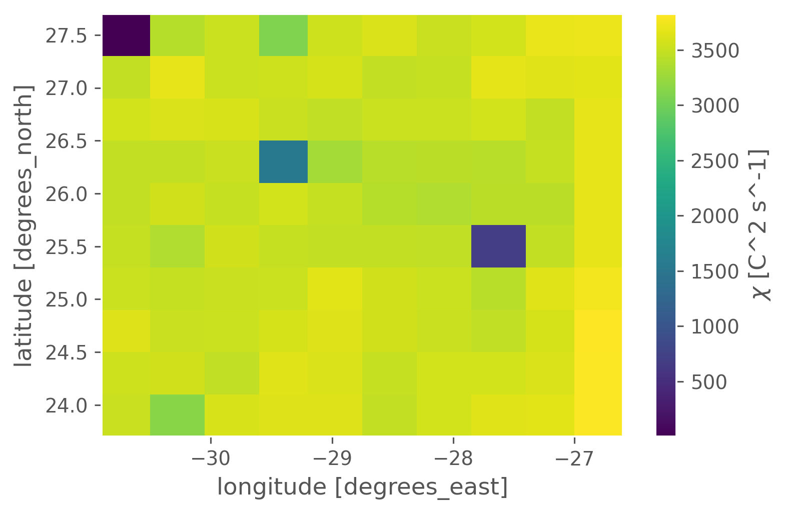
Are there any obvious sampling biases in NATRE?#
No. Just a three “bad” casts
counts = natre.chi.cf.sel(Z=slice(2000)).cf.count("Z")
counts
<xarray.DataArray 'chi' (latitude: 10, longitude: 10)>
array([[ 1, 3397, 3515, 3079, 3540, 3607, 3510, 3564, 3703, 3715],
[3468, 3690, 3514, 3528, 3578, 3468, 3495, 3668, 3634, 3661],
[3564, 3610, 3597, 3512, 3454, 3518, 3517, 3571, 3481, 3684],
[3472, 3482, 3498, 1545, 3317, 3419, 3436, 3414, 3485, 3684],
[3481, 3556, 3491, 3569, 3491, 3407, 3369, 3424, 3429, 3689],
[3490, 3375, 3551, 3492, 3470, 3468, 3462, 697, 3475, 3682],
[3514, 3493, 3511, 3525, 3648, 3549, 3518, 3419, 3641, 3757],
[3624, 3509, 3522, 3575, 3627, 3551, 3510, 3458, 3581, 3826],
[3536, 3543, 3463, 3640, 3616, 3495, 3566, 3562, 3613, 3805],
[3503, 3139, 3587, 3625, 3621, 3478, 3571, 3639, 3653, 3797]])
Coordinates:
* latitude (latitude) float64 27.5 27.1 26.7 26.3 ... 25.1 24.7 24.3 23.9
* longitude (longitude) float64 -30.7 -30.3 -29.8 -29.4 ... -27.6 -27.2 -26.8
time (latitude, longitude) datetime64[ns] 1992-03-28T15:28:59.99999...
Attributes:
long_name: $χ$
standard_name: ocean_dissipation_rate_of_thermal_variance_from_microtemp...
units: C^2 s^-1natre.chi.cf.sel(Z=slice(2000)).cf.count("Z").plot()
<matplotlib.collections.QuadMesh at 0x177bd0280>
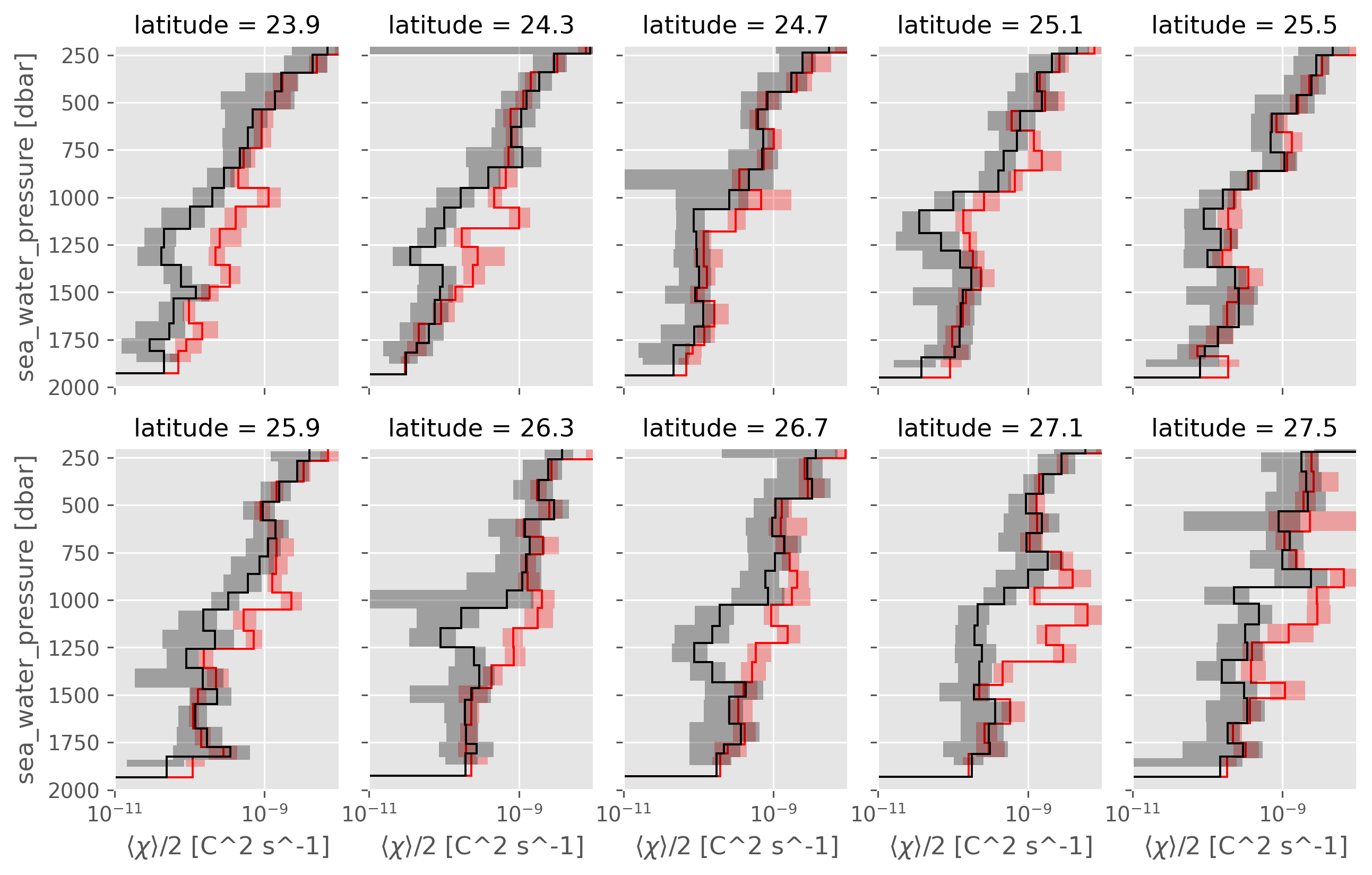
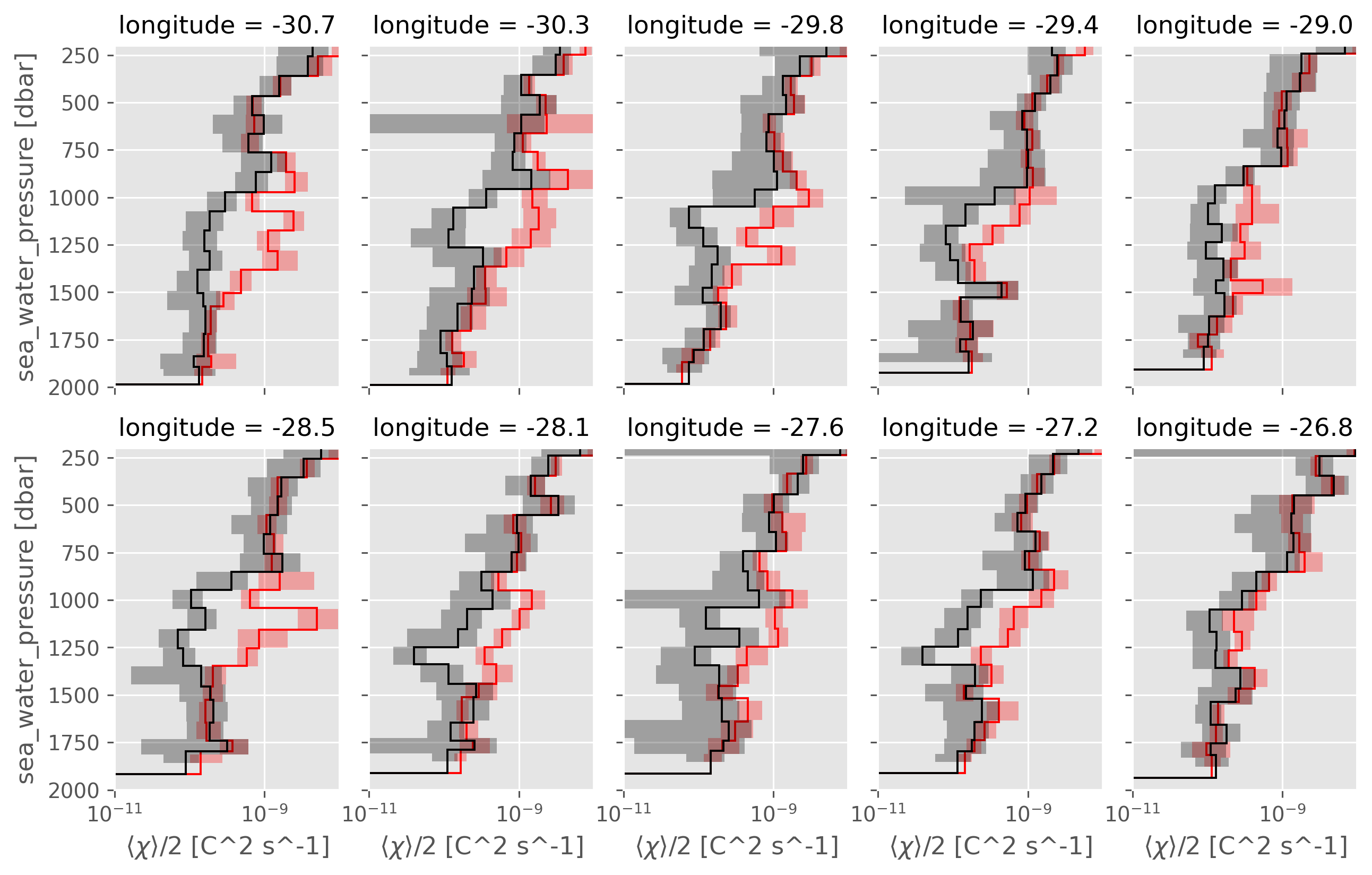
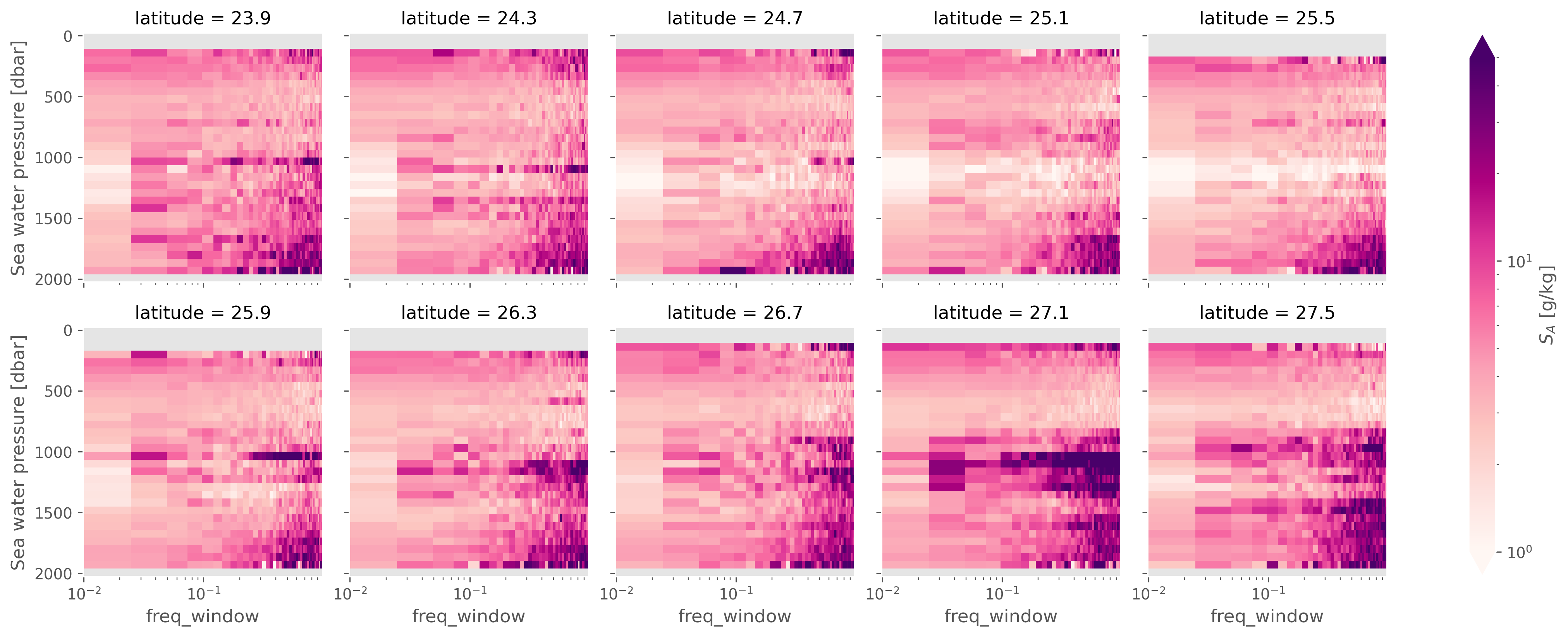
NATRE latitudinal and longitudinal lines#
Interestingly, most “lines” do show eddy stirring : ~ 6/10 panels in the following figure.
So it does seem like a single CTD-χpod section has some chance of replicating that result.
A05 is 24.5°N, which might not be the right “place” :( but why? How can we double check this
ed.natre.plot_lines(latlines, col="latitude")
ed.natre.plot_lines(lonlines, col="longitude")
<xarray.plot.facetgrid.FacetGrid at 0x1732266d0>
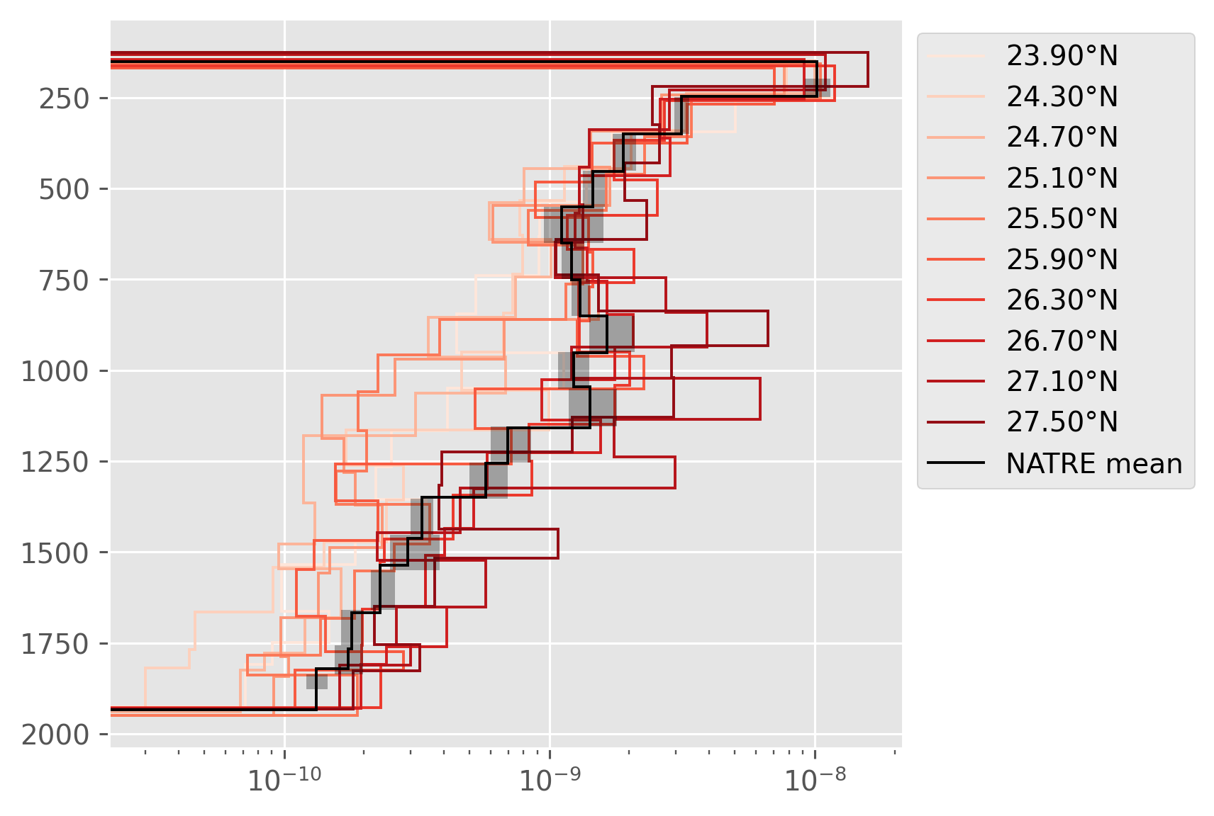
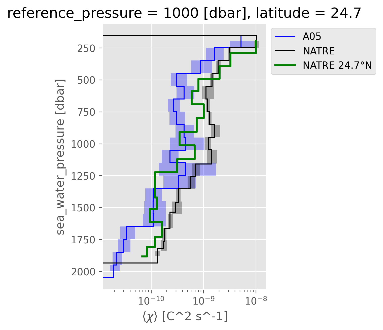
Compare 24.7°N#
NATRE data along 24.7 line is definitely lower than the NATRE mean, but not as low as CTD-χpod.
Is it possible that this latitude is just a bad place? A05 could have missed the signal, but how can we tell for sure?
A05: There is T-S spread.
A05: Higher χ values are to the east. Adding cast 131 which looks like a Meddy outlier makes a big difference
~Could use Argo to map mean spice field~ Mean spice field has basin-wide high values in 750m-1250m zone
(
latlines.chib2.hvplot.step(y="pres", by="latitude", muted_alpha=0)
* natre_binned.chib2.hvplot.step(y="pres", color="k", line_width=4, label="NATRE")
* a05_binned_old.chib2.hvplot.step(
y="pres", color="b", line_width=4, label="A05 w/ 131"
)
* a05_binned.chib2.hvplot.step(
y="pres", color="g", line_width=4, label="A05 110-129"
)
).opts(
ylim=(2000, 0),
logx=True,
frame_height=500,
frame_width=250,
xlim=(1e-11, 1e-8),
show_grid=True,
)
with plt.rc_context({"axes.prop_cycle": dcpy.plots.cmap_color_cycler()}):
f, ax = plt.subplots(1, 1, constrained_layout=True)
# 0.5m * 200 ~ 100m resolution
# (natre.mean("longitude").cf.coarsen(Z=200, boundary="trim").mean().chi / 2).cf.plot(
# hue="latitude", xscale="log", zorder=0, lw=1
# )
for lat in latlines.latitude:
dcpy.plots.fill_between_bounds(
latlines.sel(latitude=lat),
"chib2",
y="pres",
label=f"{lat.data:.2f}°N",
fill=False,
)
dcpy.plots.fill_between_bounds(
natre_binned, "chib2", y="pres", color="k", label="NATRE mean"
)
ax.set_xscale("log")
ax.legend(bbox_to_anchor=(1, 1))
Compare χ profiles#
2m#
I’m not sure that this is the right “resolution”.
The CTD-χpod is technically 2m; but is quite noisy… It looks more like the 0.5m NATRE data!
kwargs = dict(
ylim=(2000, 0),
logx=True,
muted_alpha=0,
line_width=0.5,
aspect=1 / 2,
frame_width=250,
xlim=(1e-12, 1e-6),
grid=True,
)
a05_casts = chipod.cf.sel(profile_id=slice(119, 129)).chi.hvplot.line(
by="station", y="pressure", title="A05", **kwargs
)
natre_casts = natre_2m.chi.hvplot(y="pres", by="longitude", title="NATRE", **kwargs)
(a05_casts + natre_casts).opts(title="")
0.5m#
kwargs = dict(
ylim=(2000, 0),
logx=True,
muted_alpha=0,
line_width=0.5,
aspect=1 / 2,
frame_width=250,
xlim=(1e-12, 1e-6),
grid=True,
)
a05_casts = chipod.cf.sel(profile_id=slice(119, 129)).chi.hvplot.line(
by="station", y="pressure", title="A05", **kwargs
)
natre_casts = natre.chi.hvplot(y="pres", by="longitude", title="NATRE", **kwargs)
(a05_casts + natre_casts).opts(title="")
natre_line = latlines.sel(latitude=chipod.cf["latitude"].mean().data, method="nearest")
# dcpy.plots.fill_between_bounds(
# avg_older, "chib2", y="pres", color="r", label="A05 w/ 131"
# )
dcpy.plots.fill_between_bounds(a05_binned, "chib2", y="pres", color="b", label="A05")
dcpy.plots.fill_between_bounds(
natre_binned, "chib2", y="pres", color="k", label="NATRE"
)
(natre_line.chi / 2).cf.plot.step(lw=2, color="g", y="pres", label="NATRE 24.7°N")
plt.legend(bbox_to_anchor=(1, 1))
plt.xscale("log")
plt.gcf().set_size_inches((3, 5))
natre_line = latlines.sel(latitude=a05_binned.latitude.mean().data, method="nearest")
# dcpy.plots.fill_between_bounds(
# avg_older, "chib2", y="pres", color="r", label="A05 w/ 131"
# )
dcpy.plots.fill_between_bounds(a05_binned, "chib2", y="pres", color="b", label="A05")
dcpy.plots.fill_between_bounds(
natre_binned, "chib2", y="pres", color="k", label="NATRE"
)
(natre_line.chi / 2).cf.plot.step(lw=2, color="g", y="pres", label="NATRE 24.7°N")
plt.legend(bbox_to_anchor=(1, 1))
plt.xscale("log")
plt.gcf().set_size_inches((3, 5))
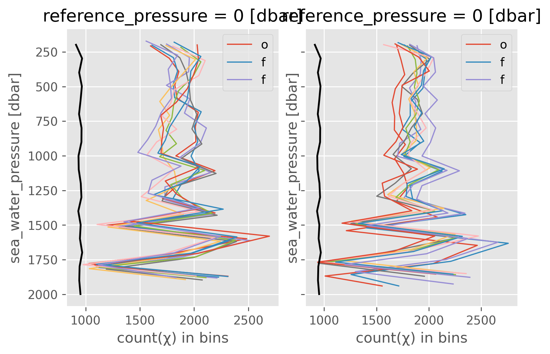
Number of observations#
This is going to depend on the input data “resolution”
f, ax = plt.subplots(1, 2, sharey=True, constrained_layout=True)
latlines.num_obs.cf.plot(hue="latitude", y="pres", ax=ax[0], lw=1)
lonlines.num_obs.cf.plot(hue="longitude", y="pres", ax=ax[1], lw=1)
for axx in ax:
a05_binned.num_obs.cf.plot(y="pres", ax=axx, color="k")
ax[0].legend("off")
ax[1].legend("off")
<matplotlib.legend.Legend at 0x1723caac0>
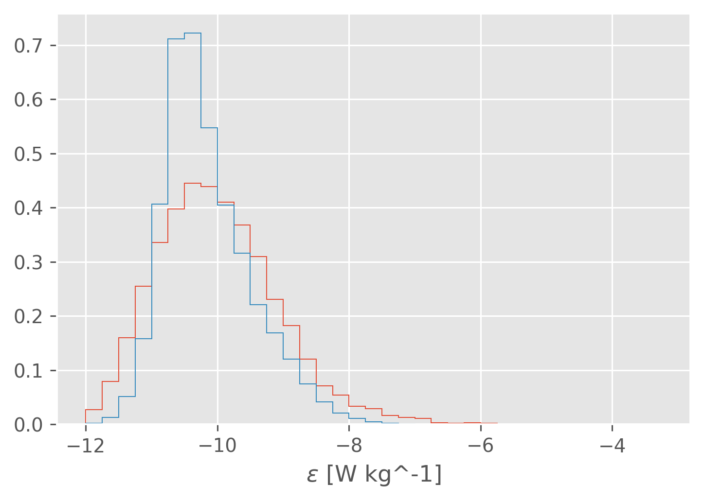
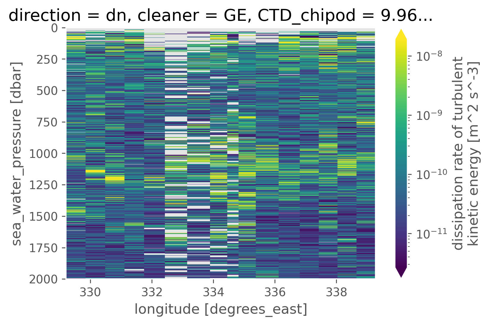
New dataset#
subset = a05.sel(station=slice(115, 130))
clean = subset["chipod"].ds.sel(cleaner="GE", direction="dn", pressure=slice(2000))
kwargs = dict(histtype="step", density=True, bins=np.arange(-12, -3, 0.25))
np.log10(clean.eps.where(np.abs(clean.dThdz) > 5e-3)).plot.hist(**kwargs, label="A05")
np.log10(natre.eps.sel(pres=slice(2000))).plot.hist(**kwargs, label="NATRE");
clean.eps.cf.plot(norm=mpl.colors.LogNorm(), robust=True)
<matplotlib.collections.QuadMesh at 0x1806a7d30>
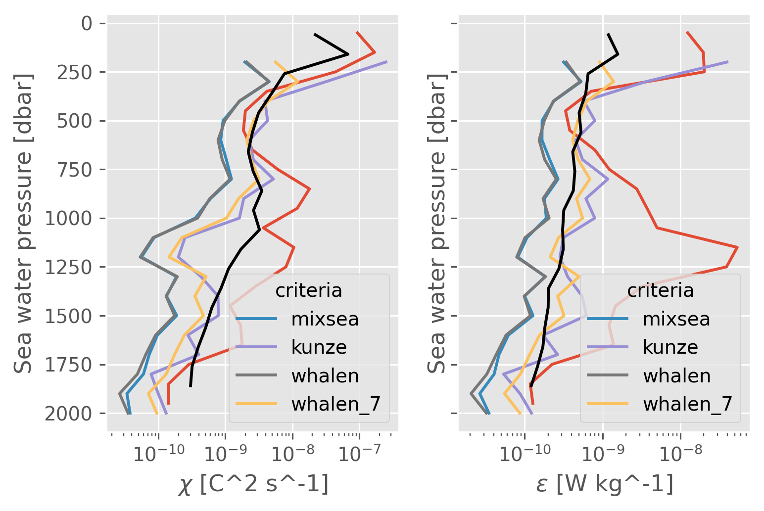
f, axx = plt.subplots(1, 2, sharey=True)
for var, ax in zip(["chi", "eps"], axx):
plt.sca(ax)
mask = np.abs(subset["chipod"].ds["dThdz"]) > 5e-3
(clean[var].coarsen(pressure=50, boundary="trim").mean().mean("station")).cf.plot(
xscale="log"
)
subset["finescale"].ds[var].sel(pressure=slice(2000)).mean("station").cf.plot(
hue="criteria", xscale="log"
)
(
natre[var]
.sel(pres=slice(2000))
.coarsen(pres=200, boundary="trim")
.mean()
.mean(["latitude", "longitude"])
.cf.plot(color="k")
)
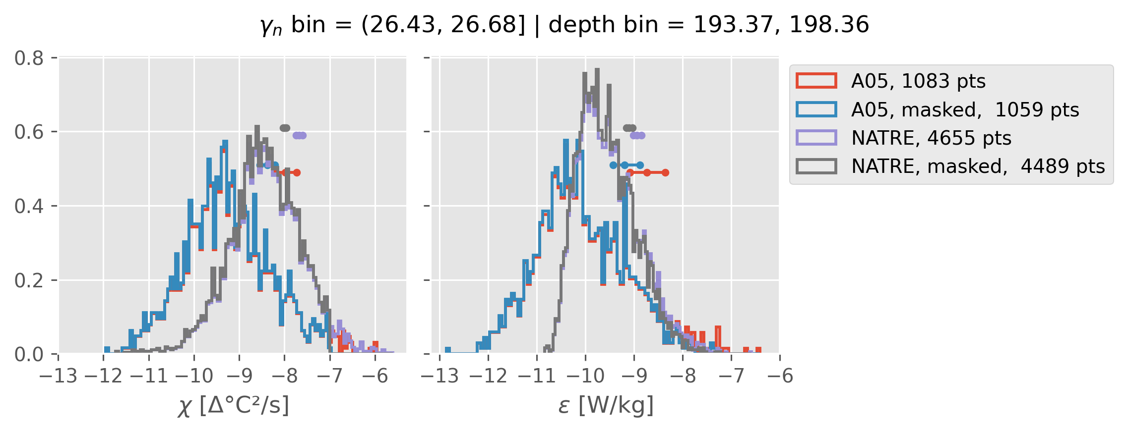
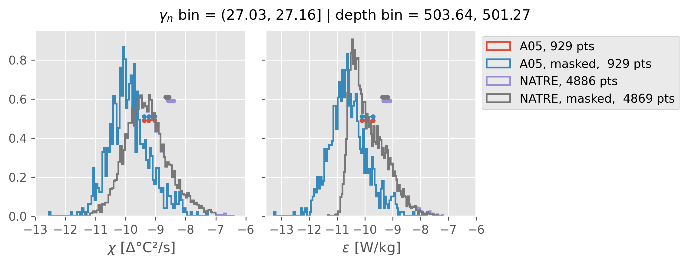
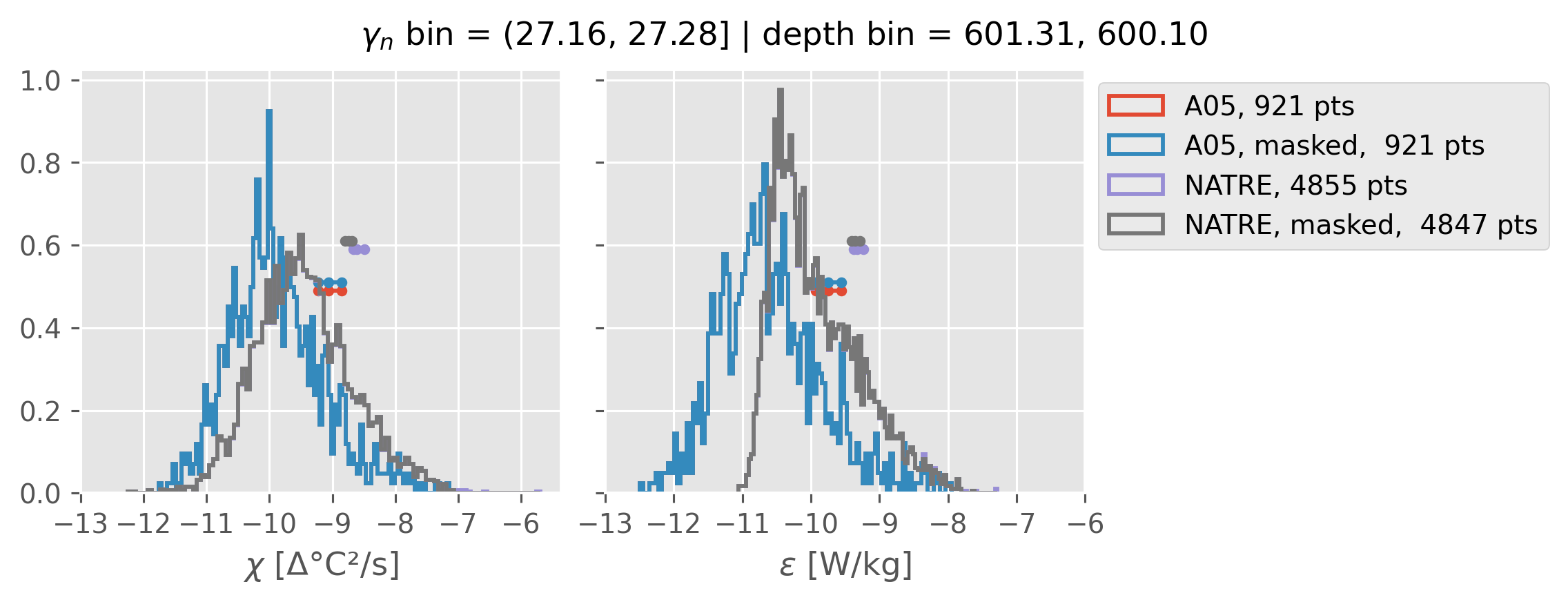
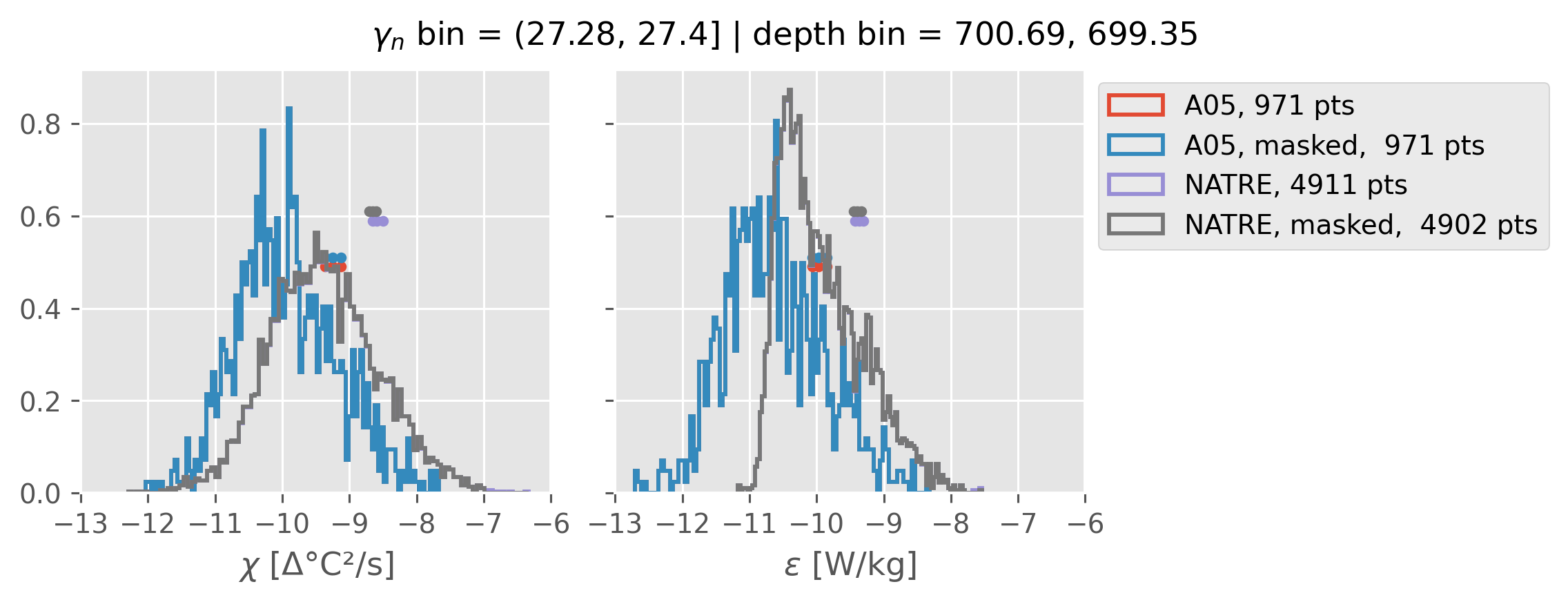
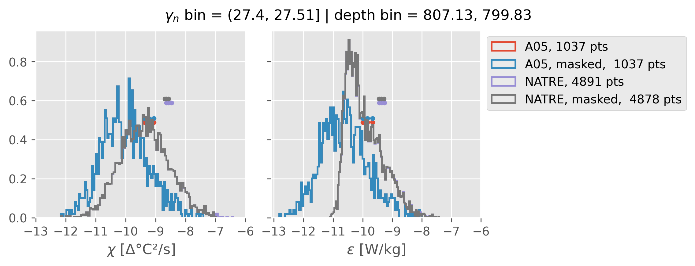
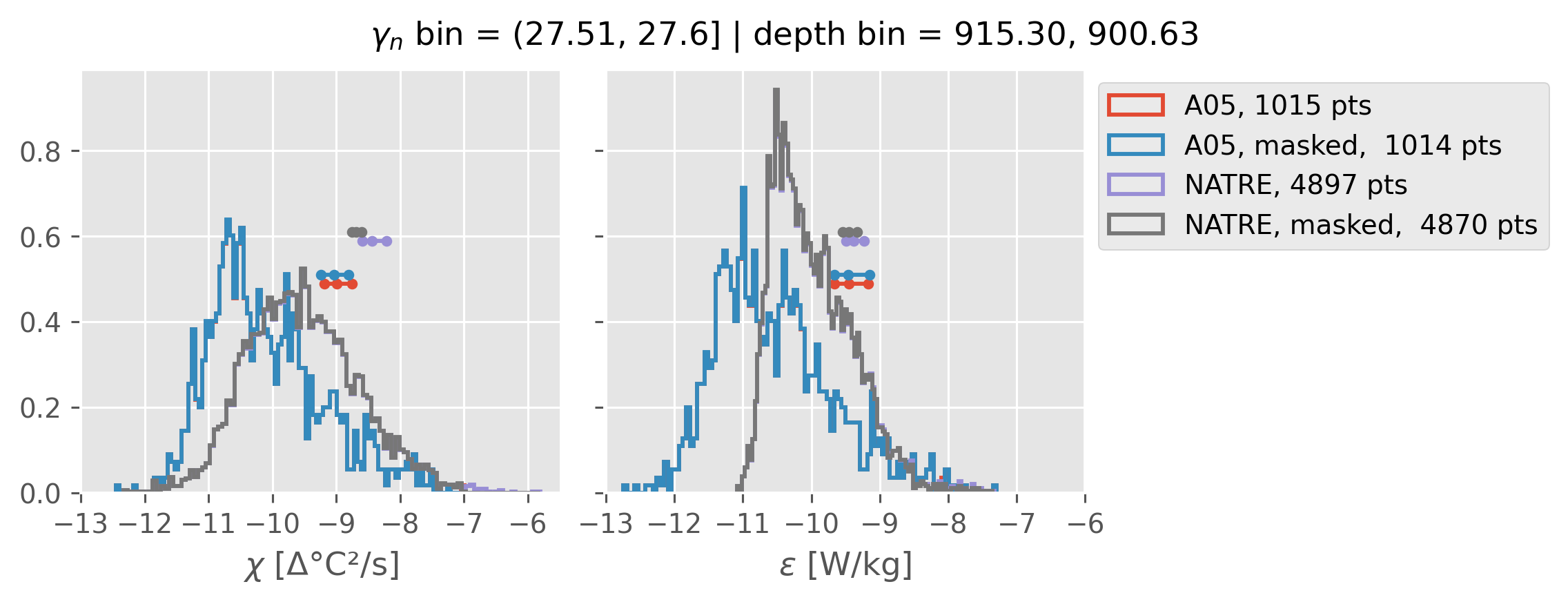
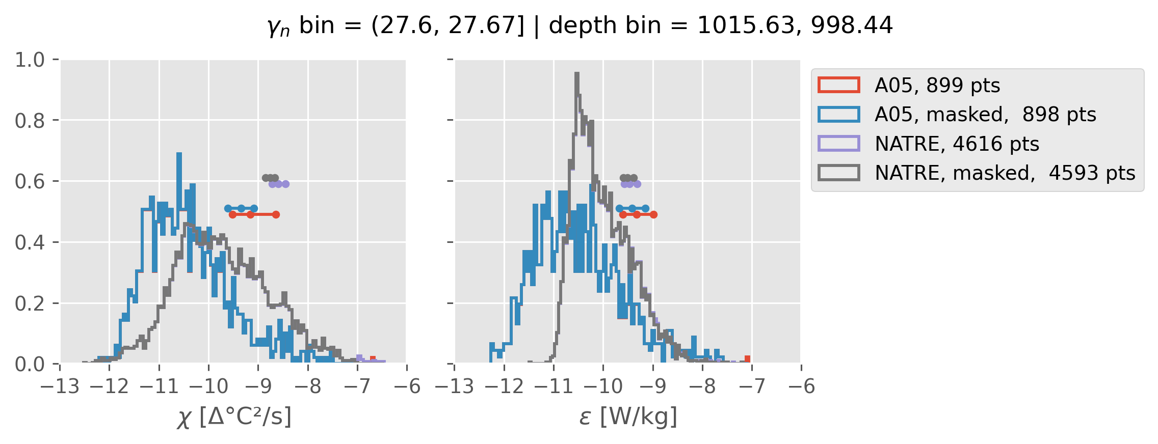
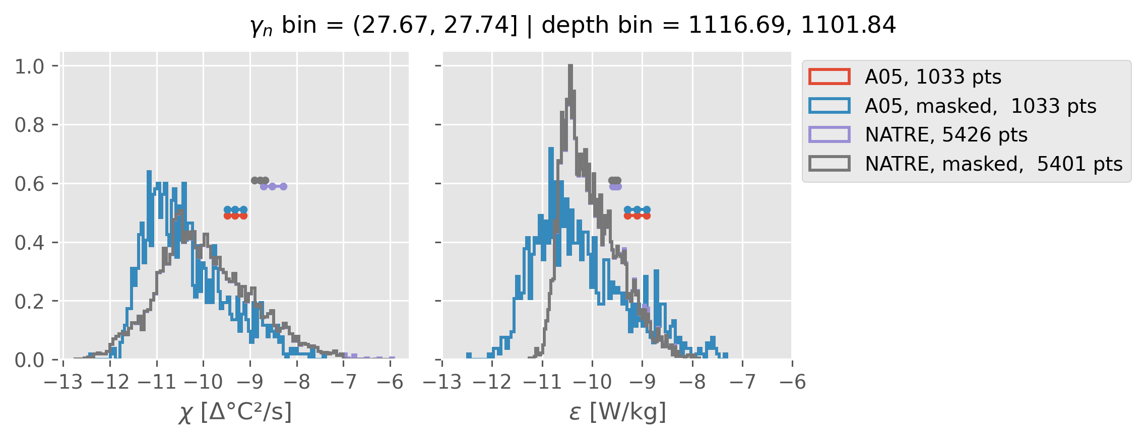
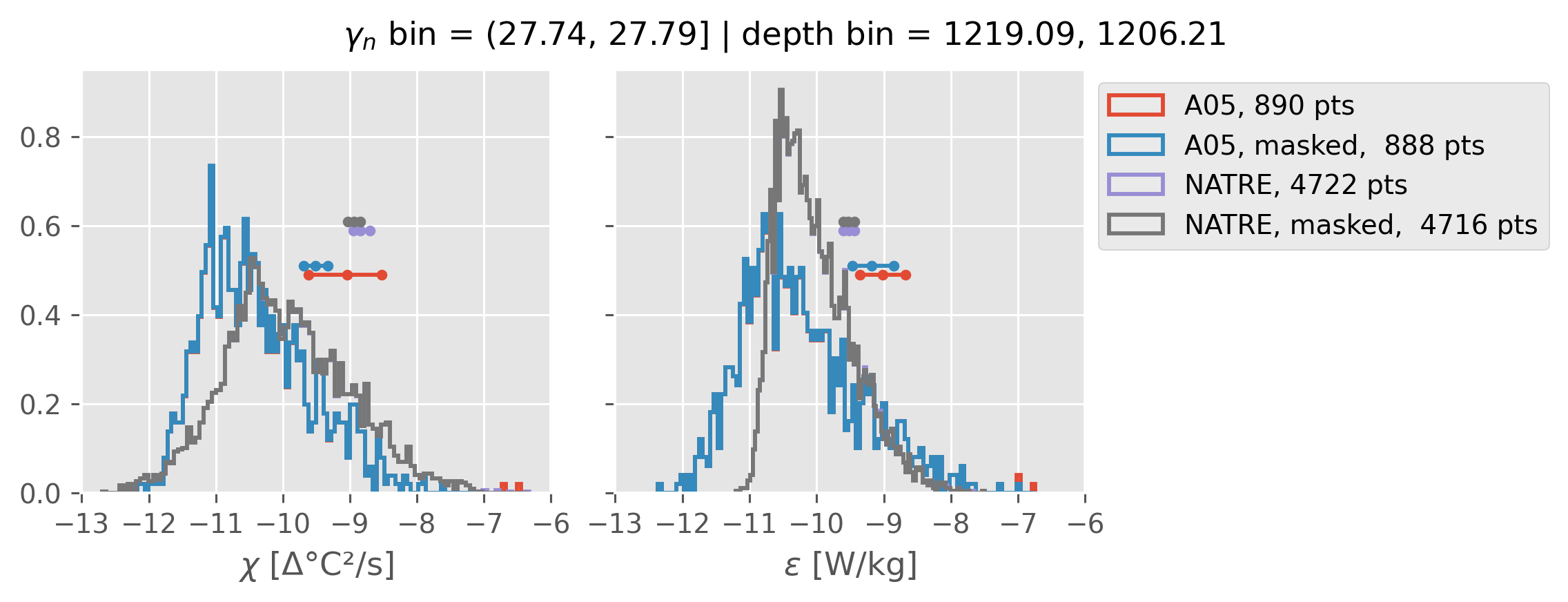
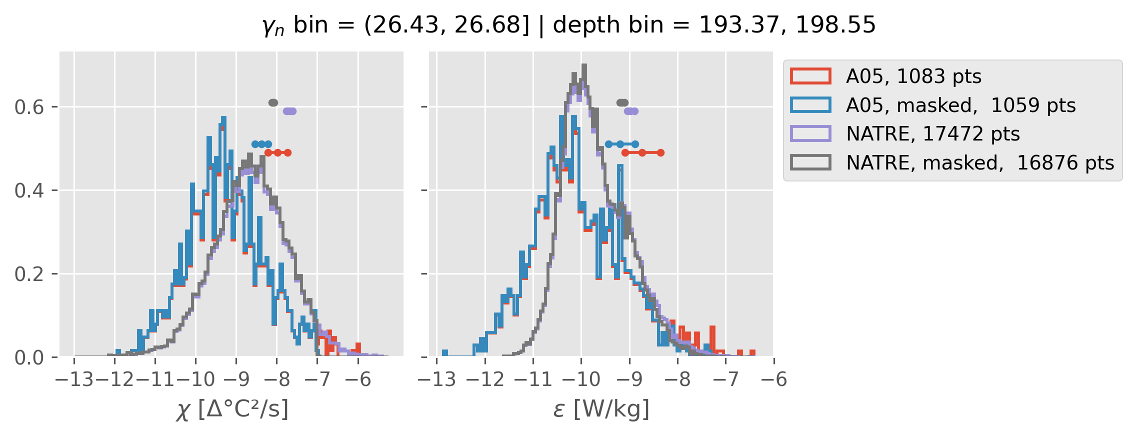
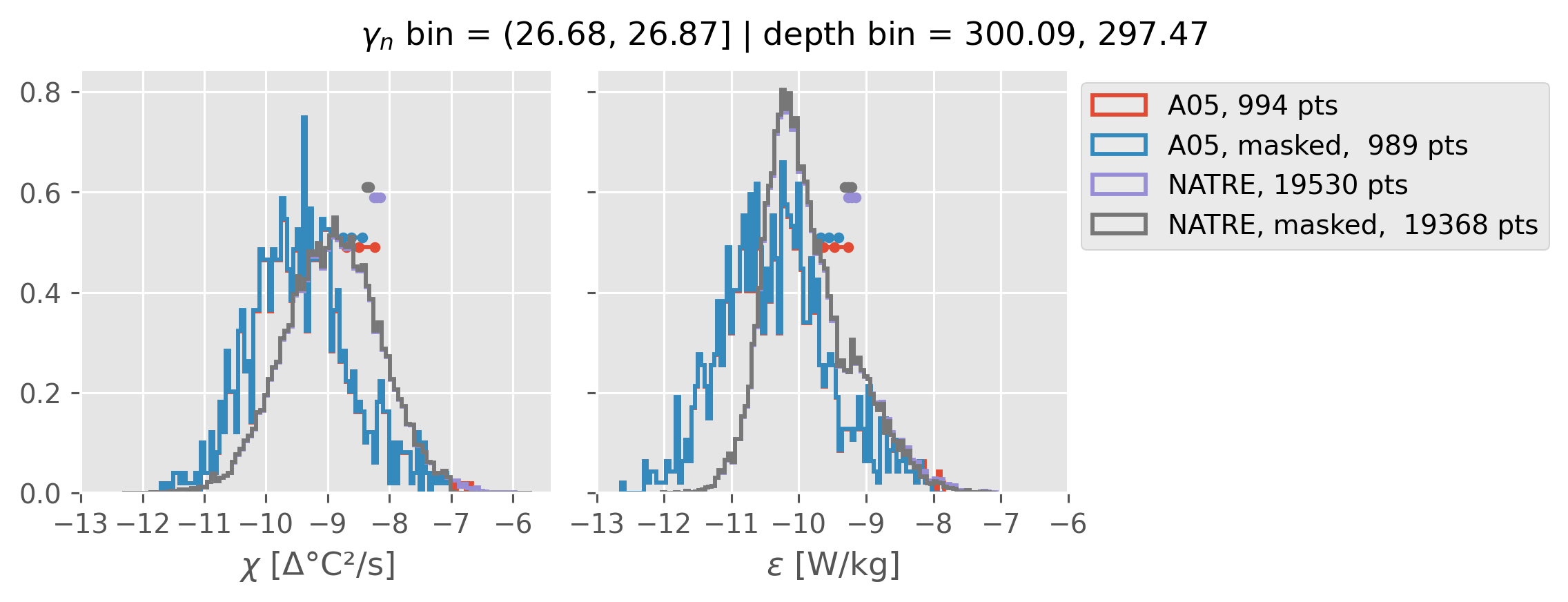
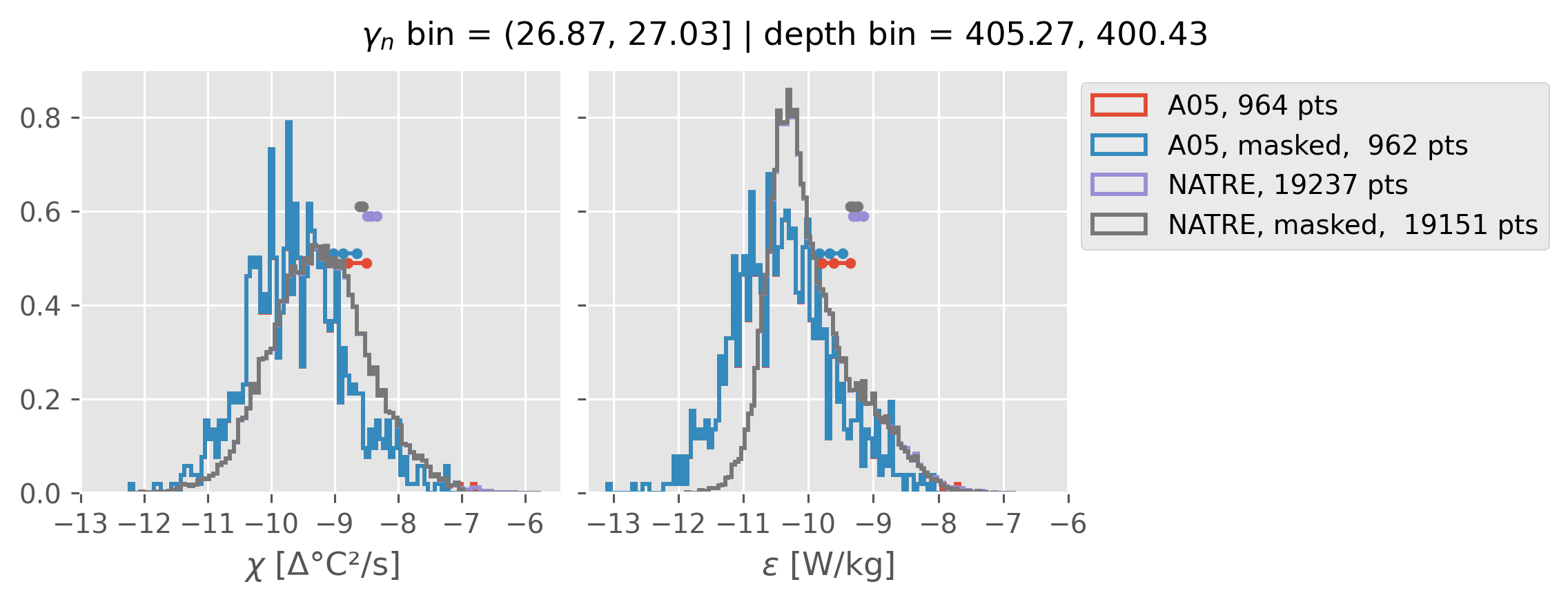
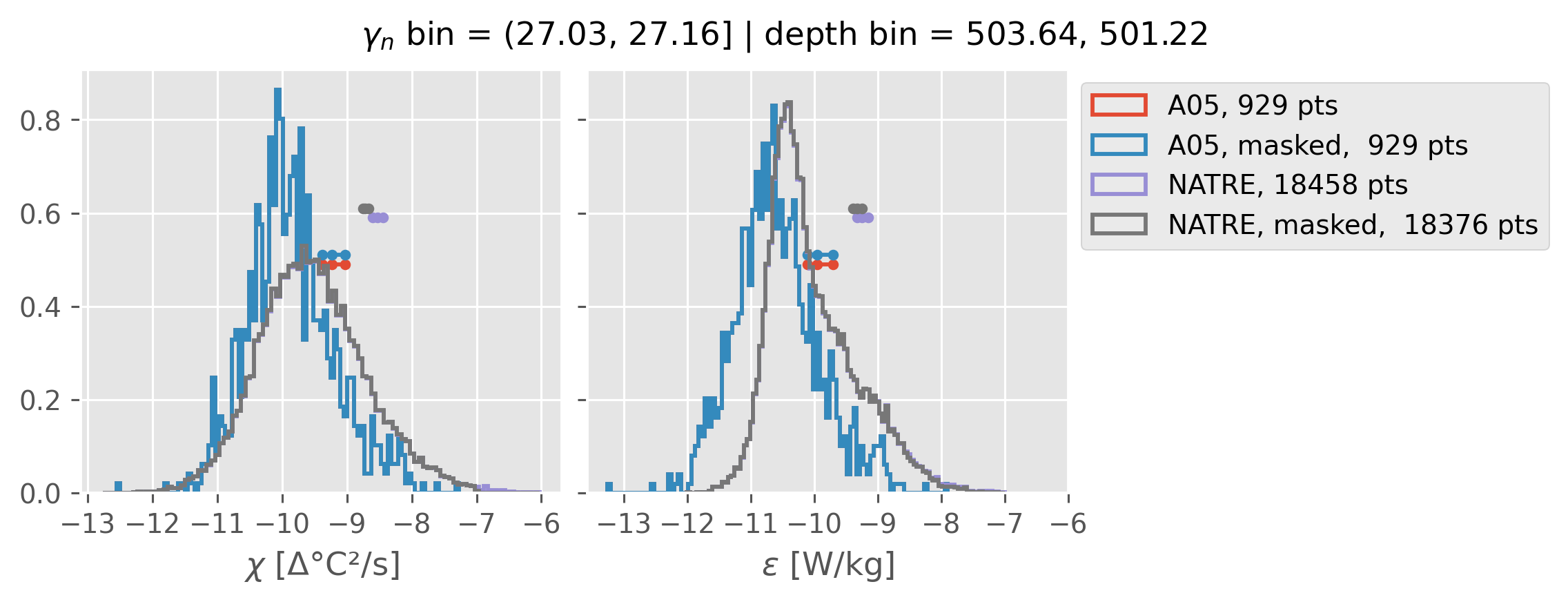
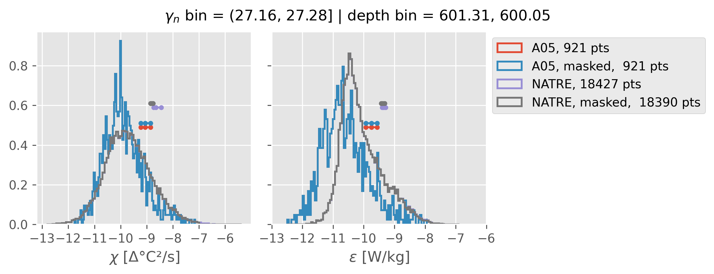
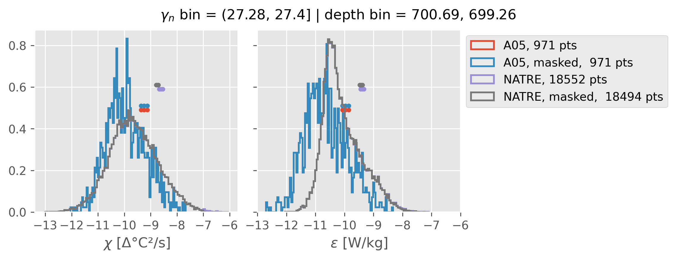
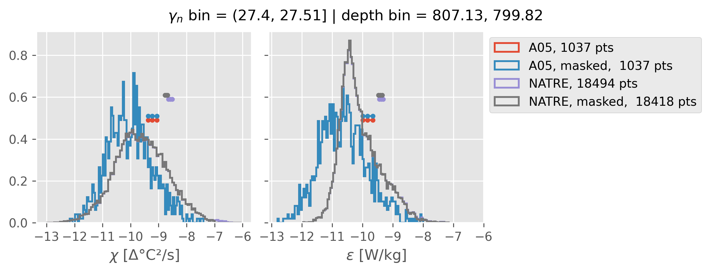
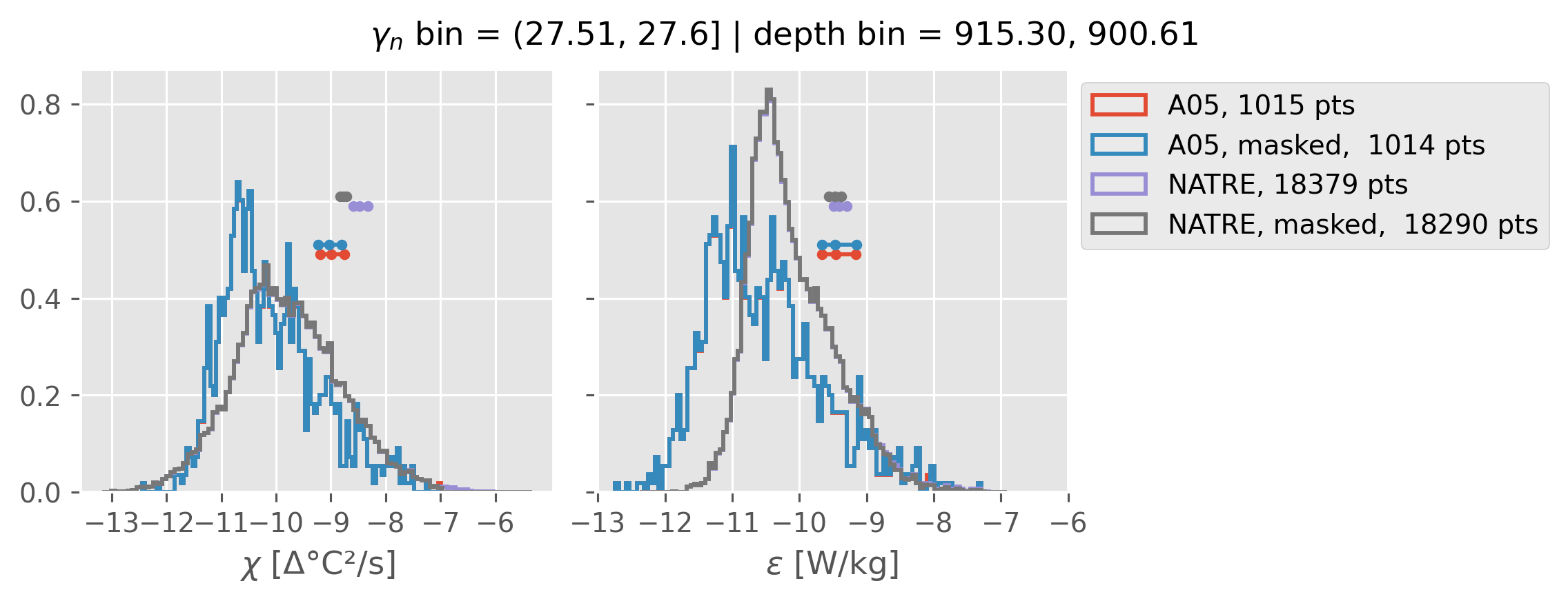
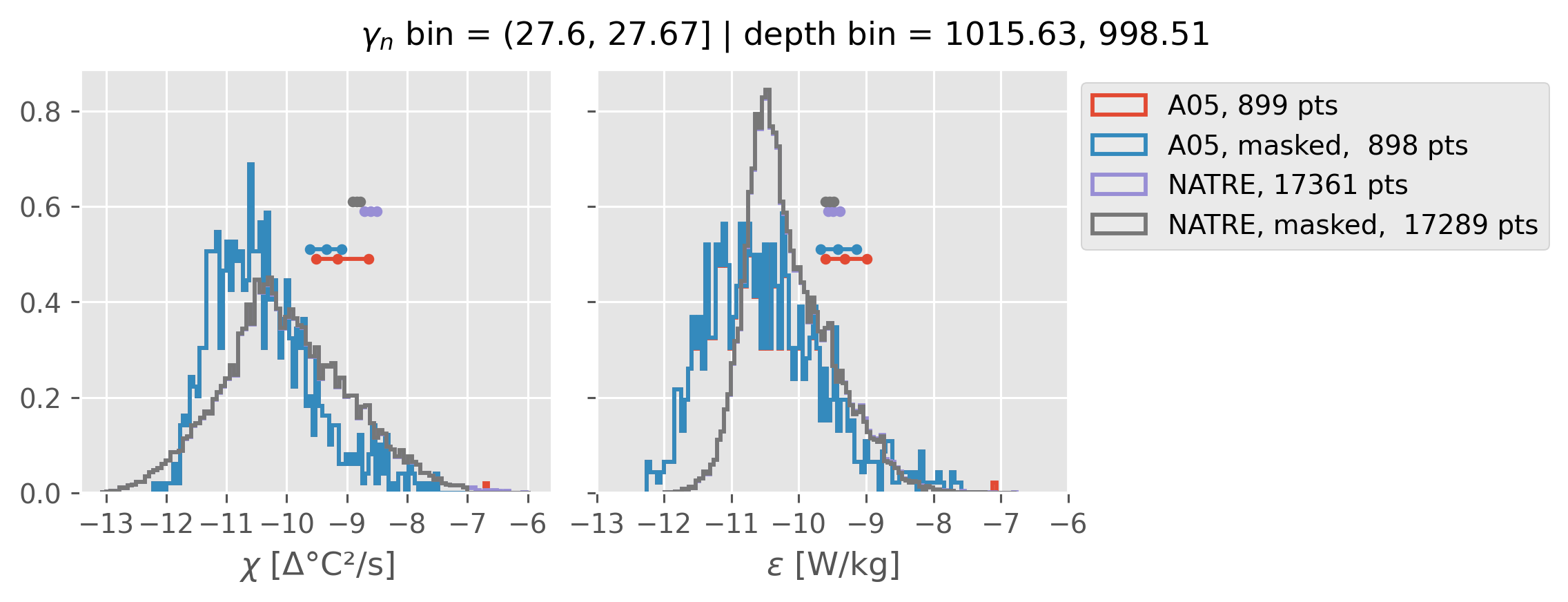
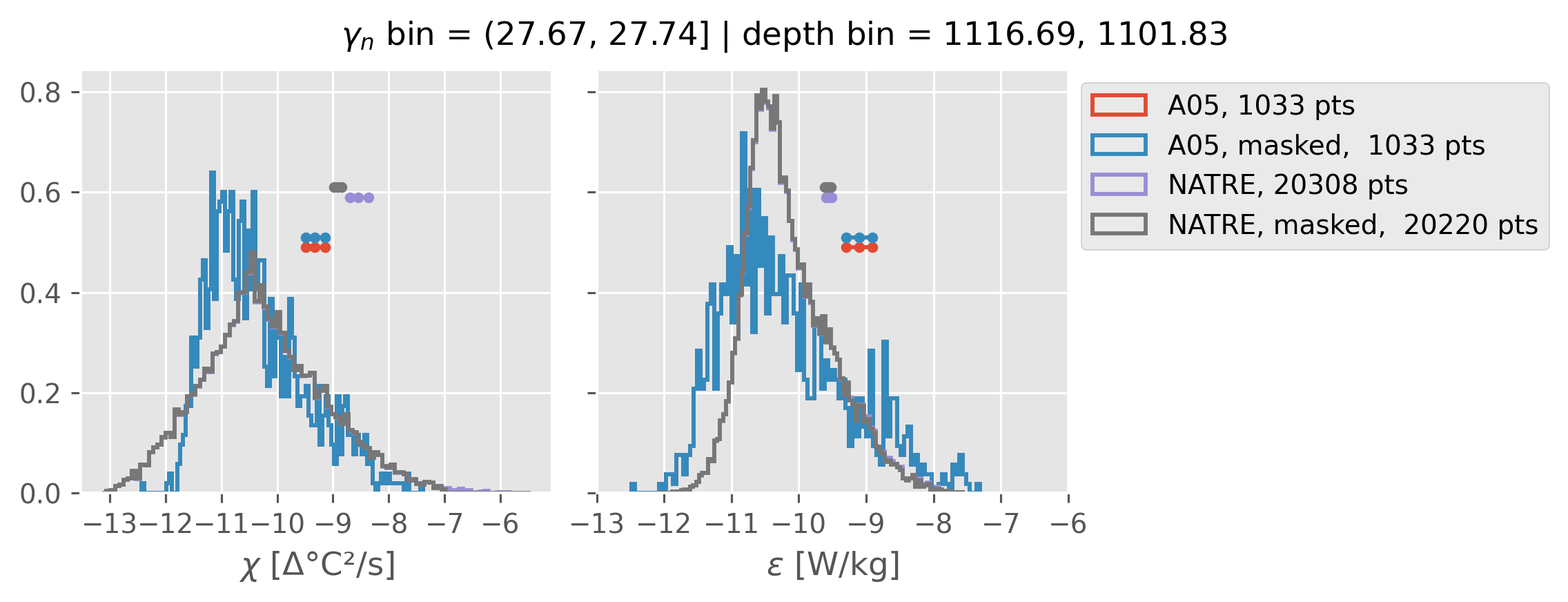
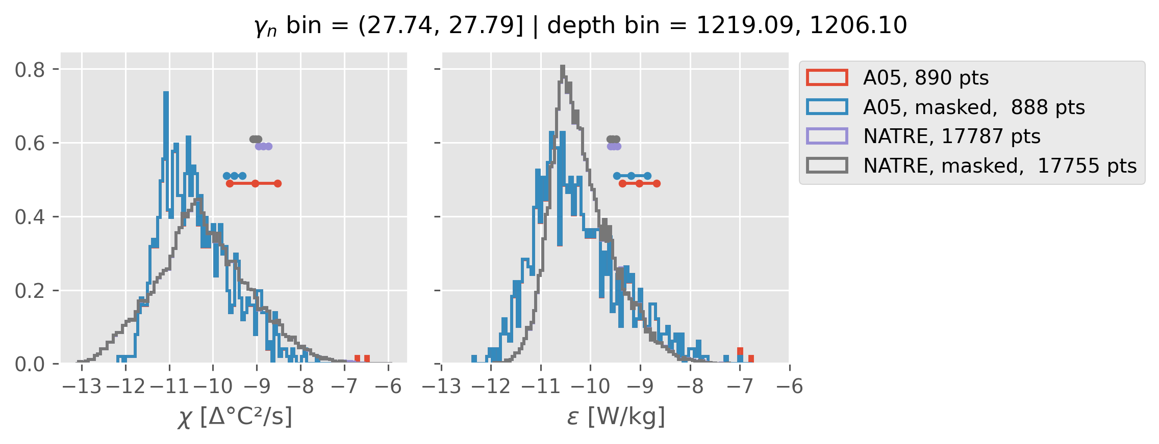
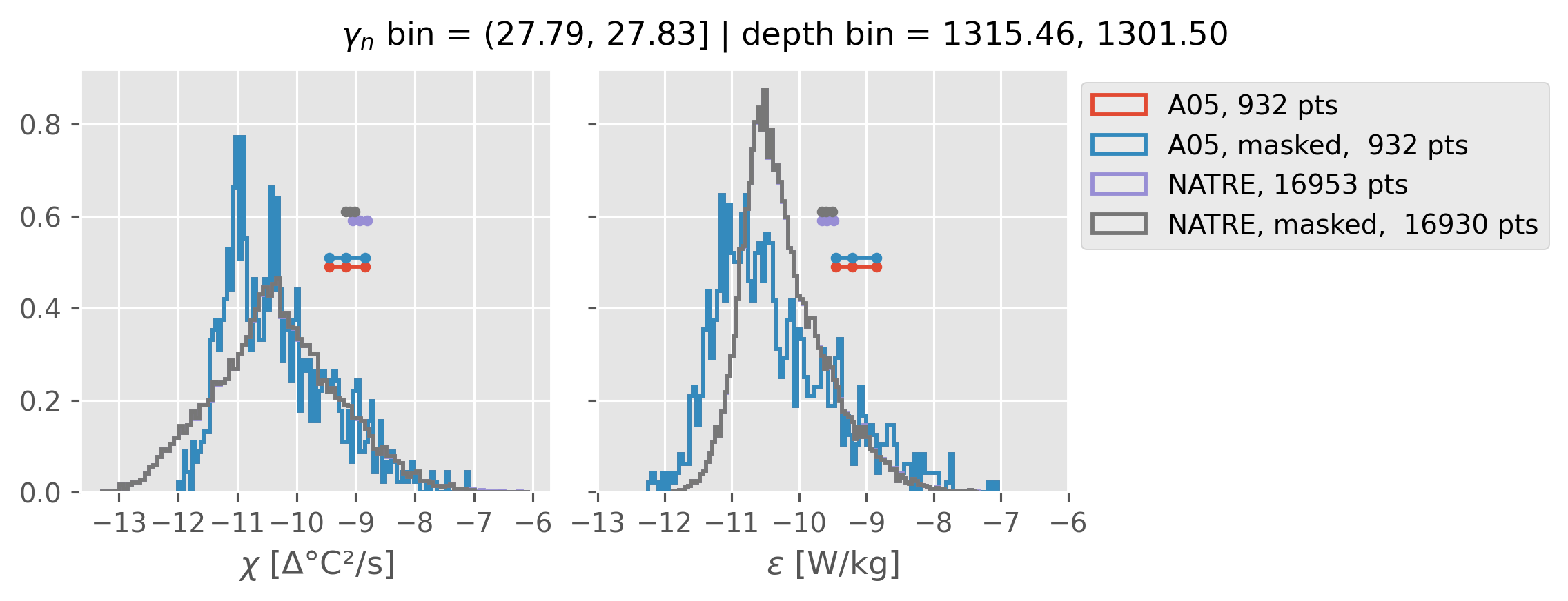
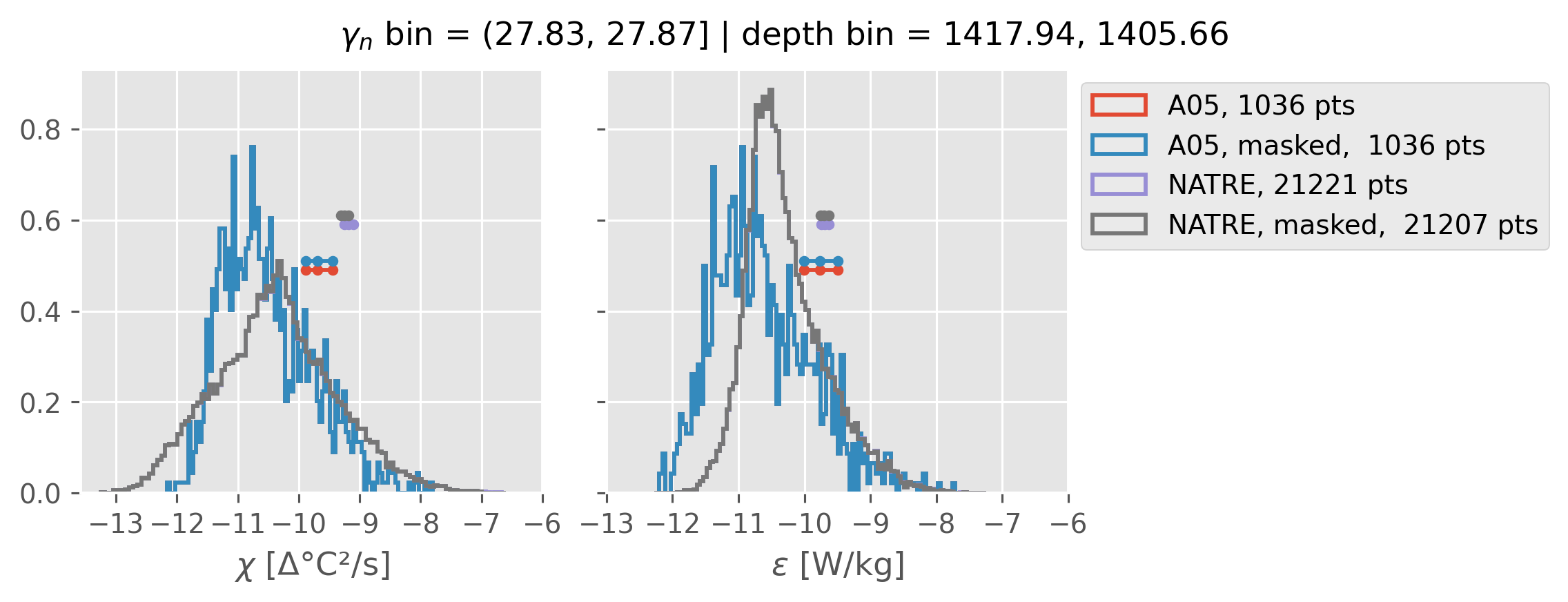
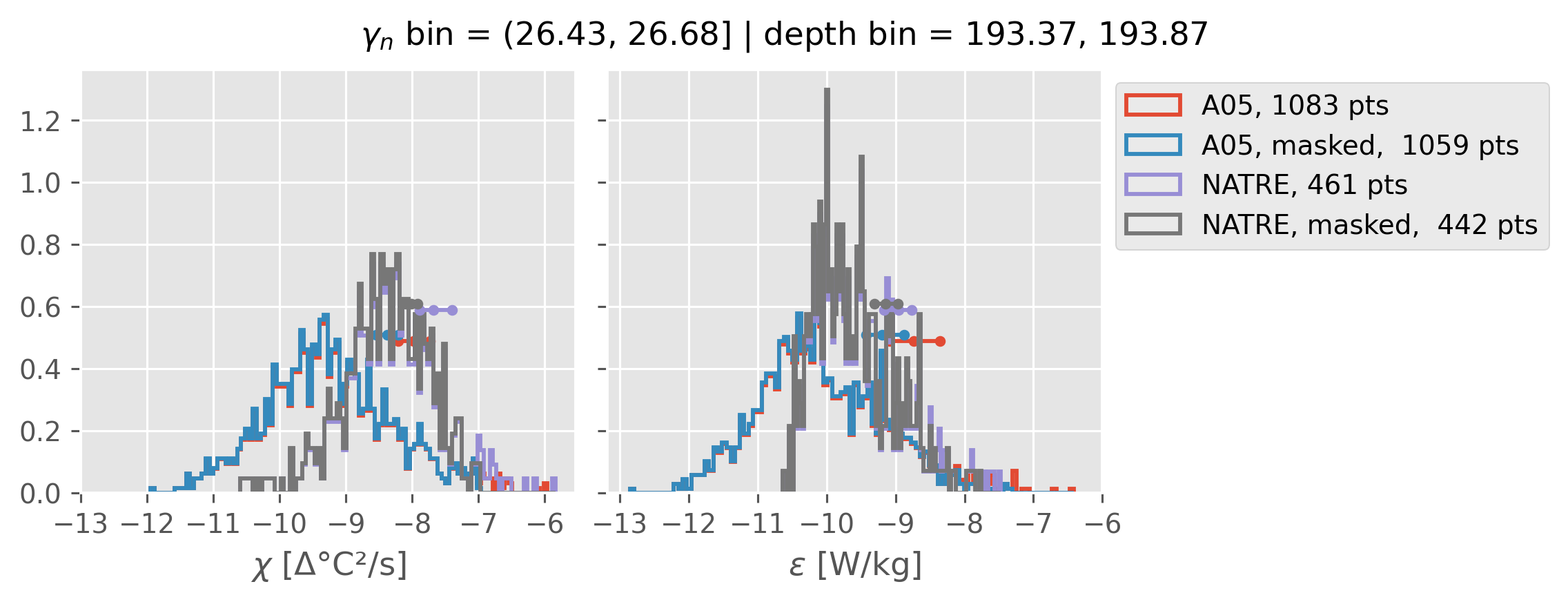
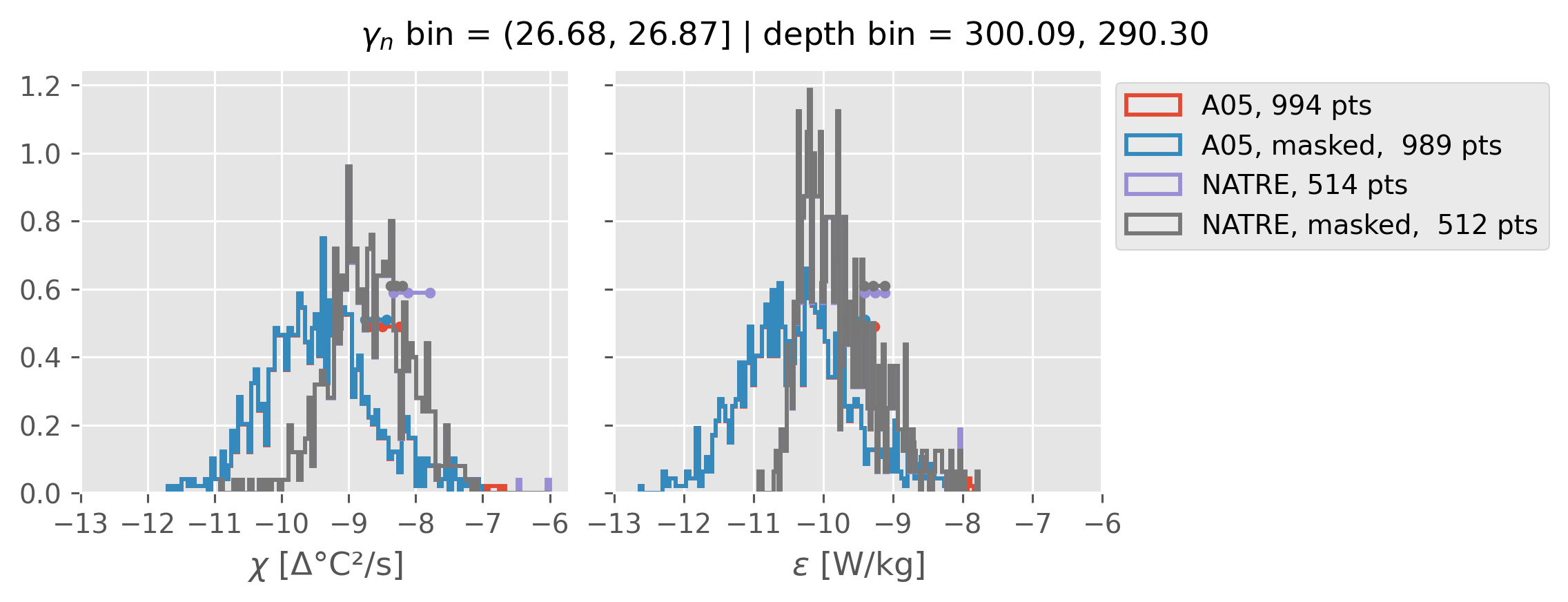
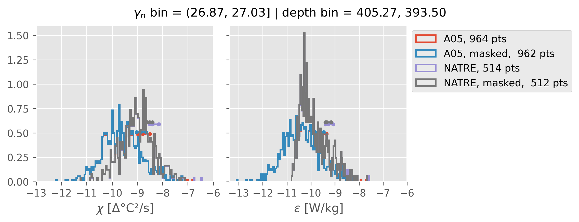
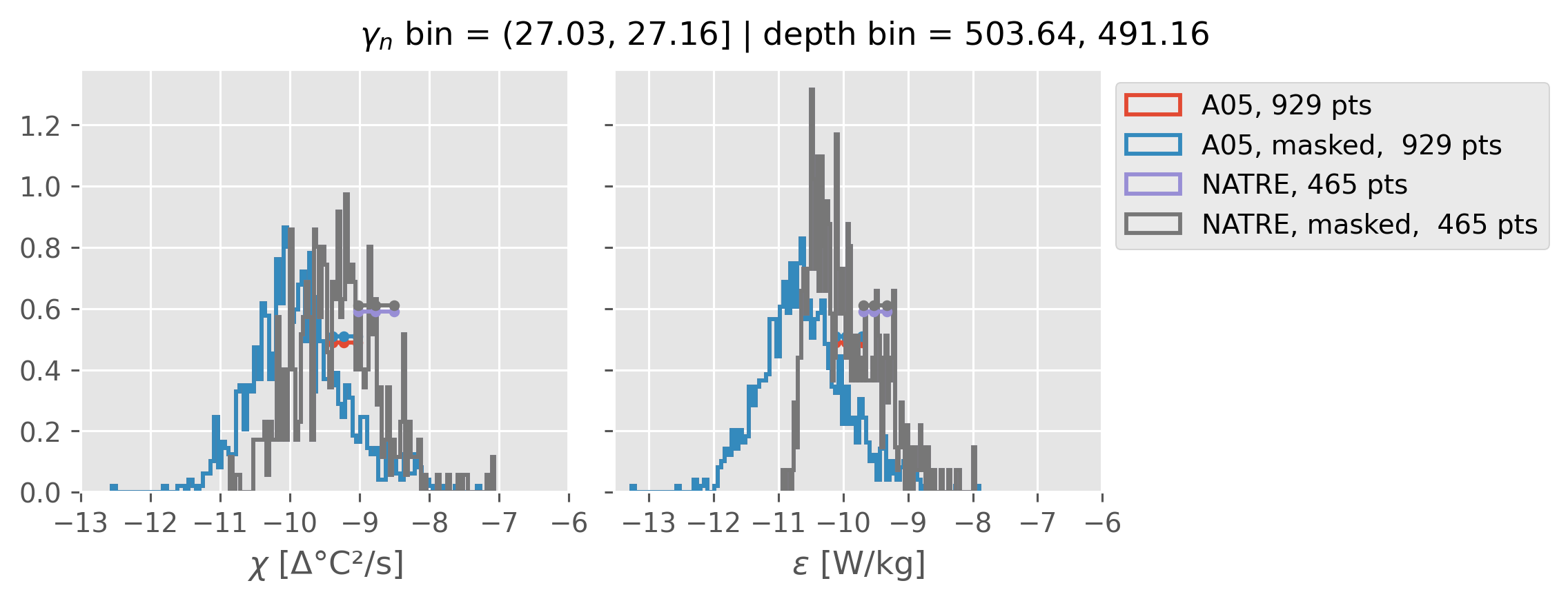
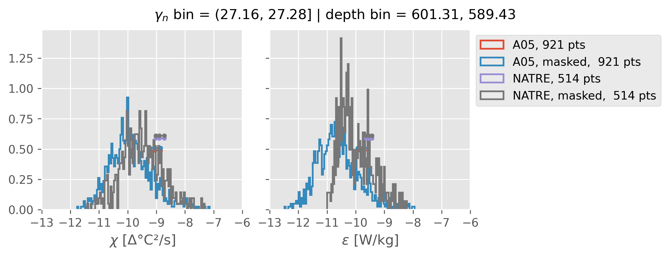
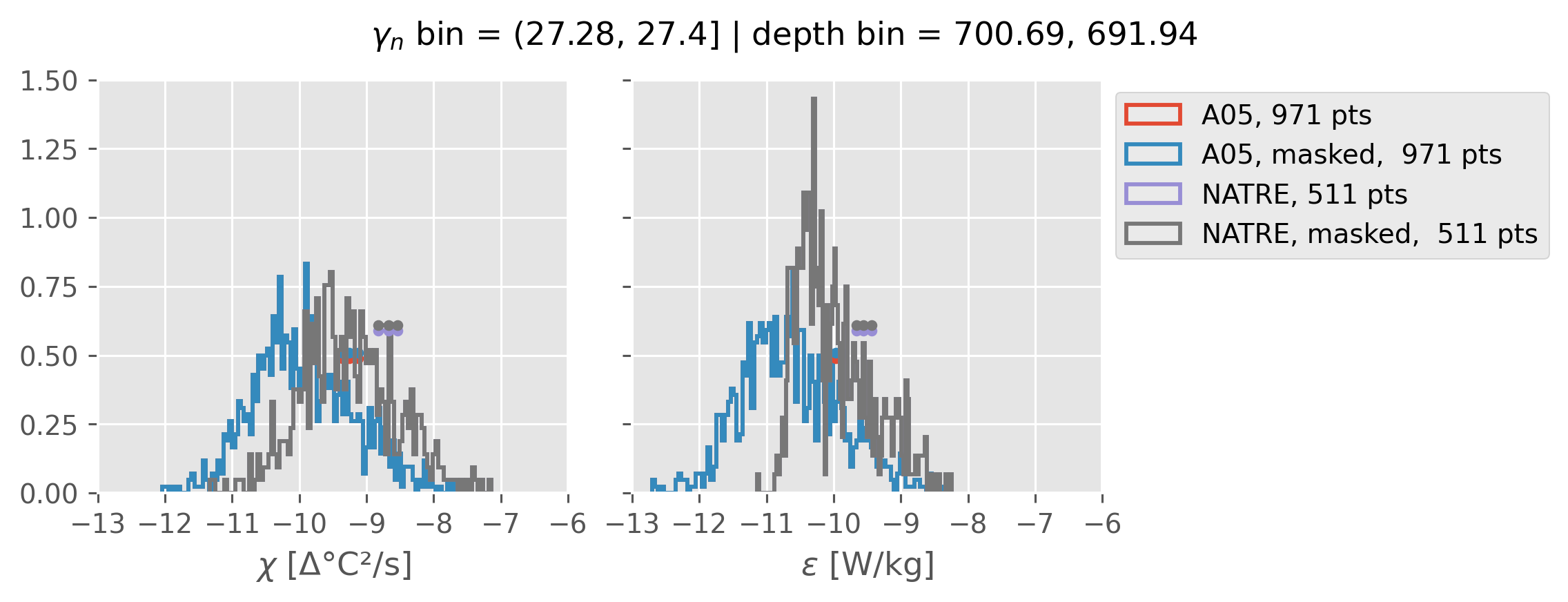
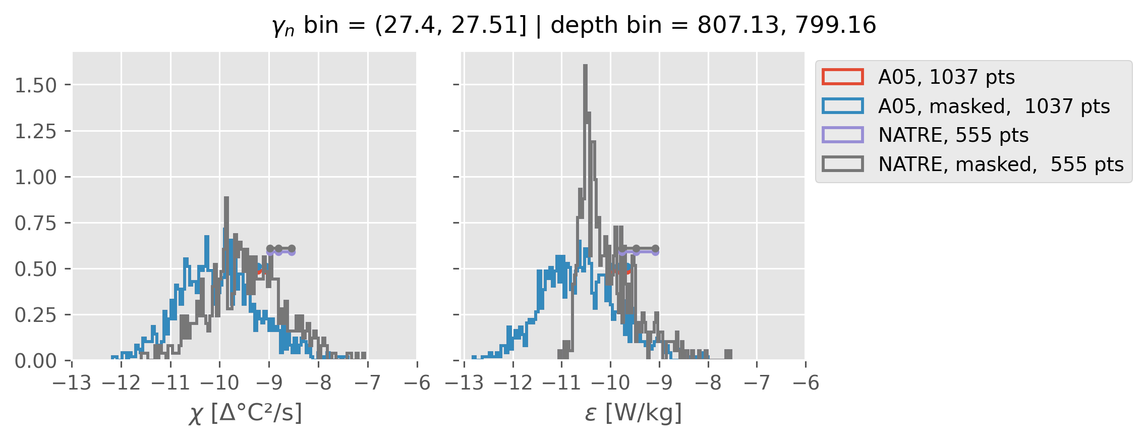
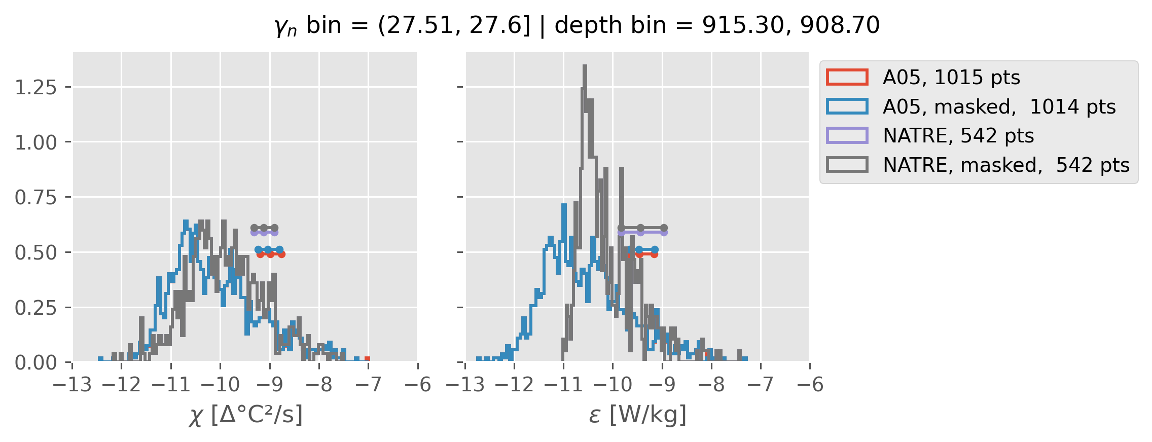
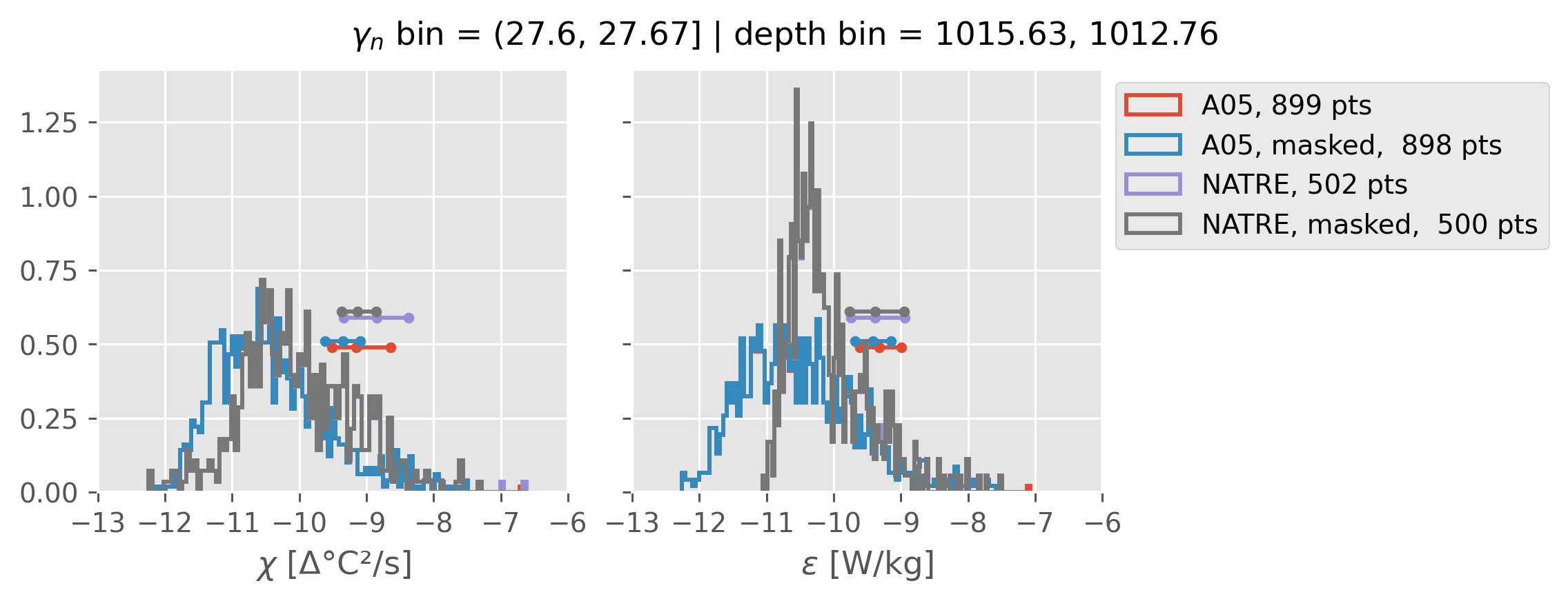
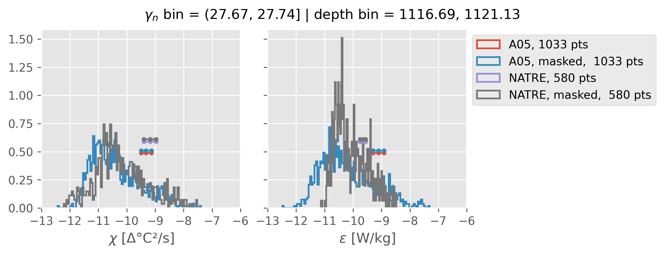
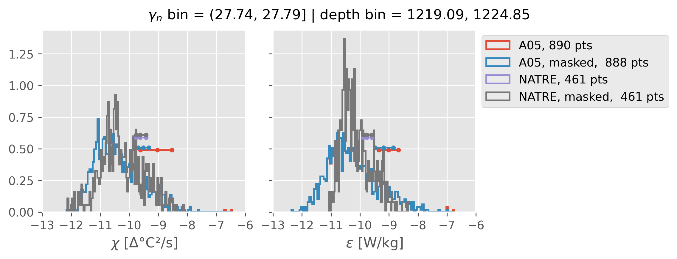
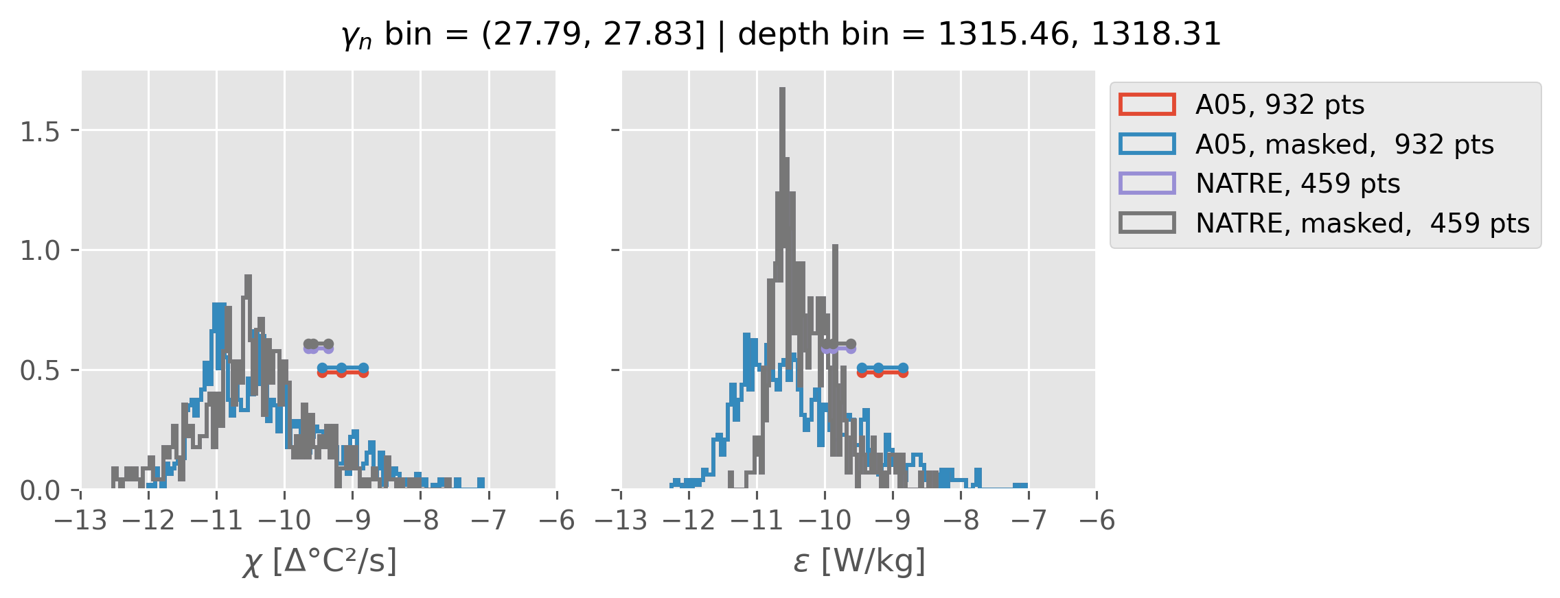
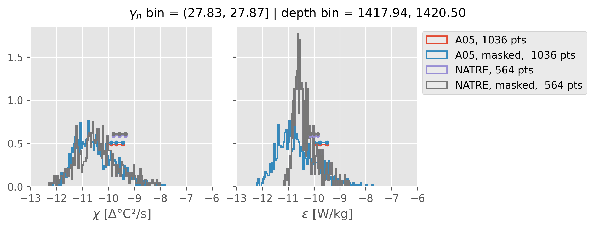
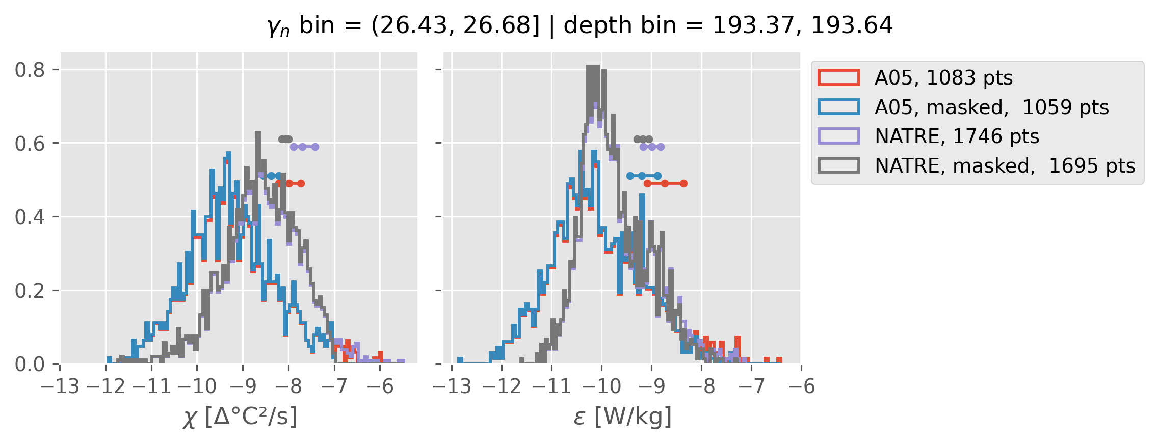
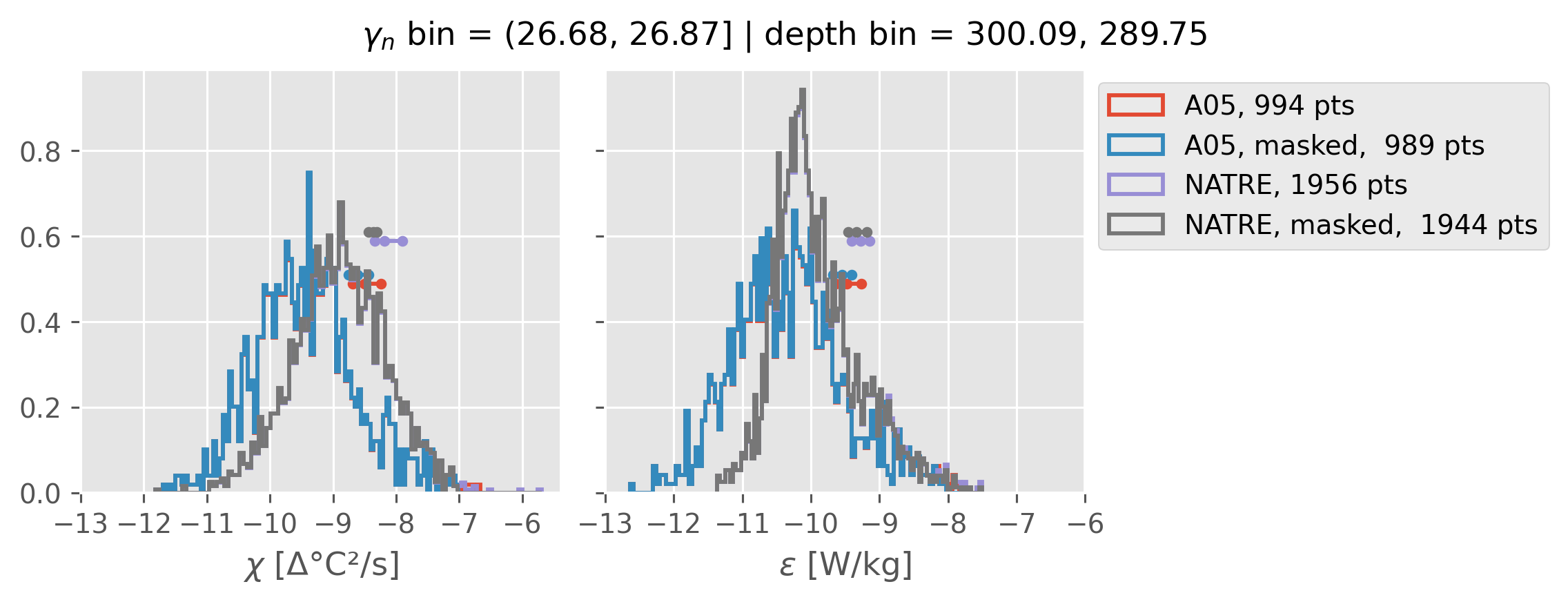
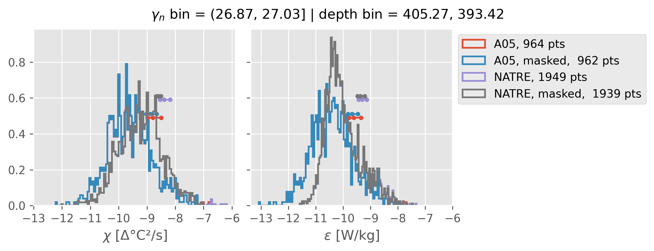
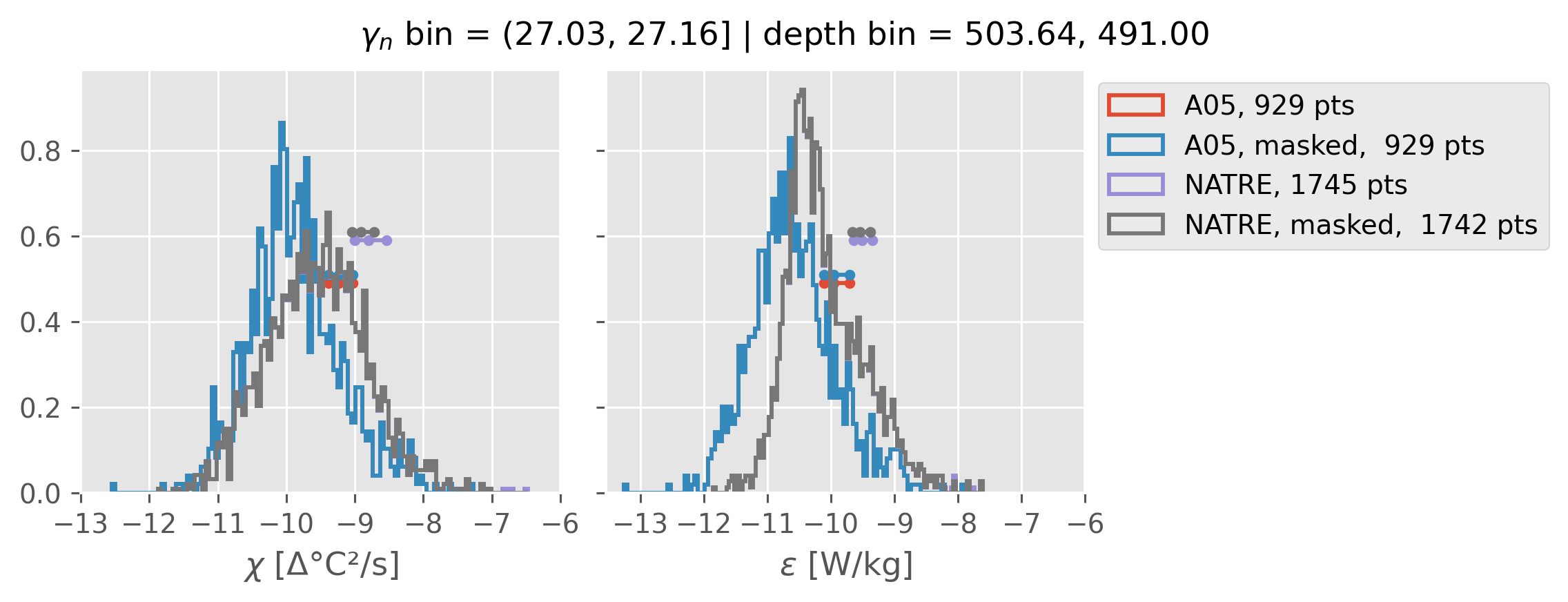
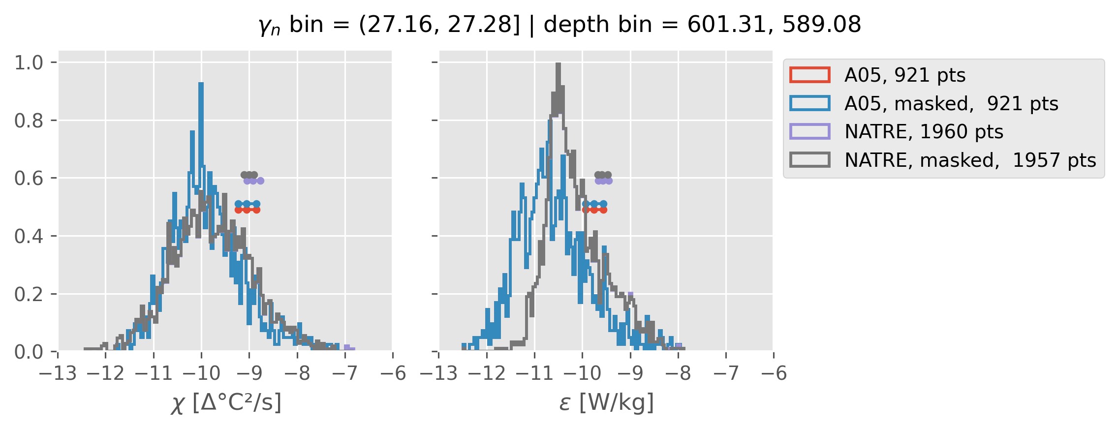
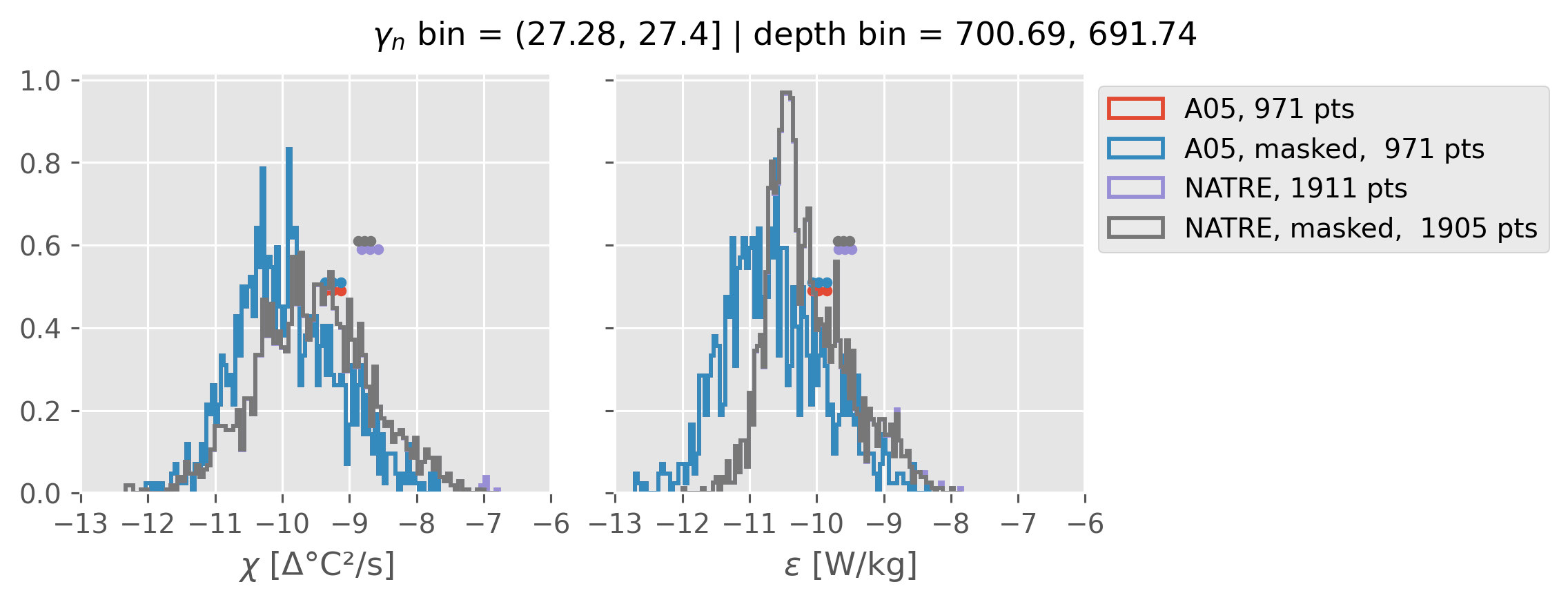
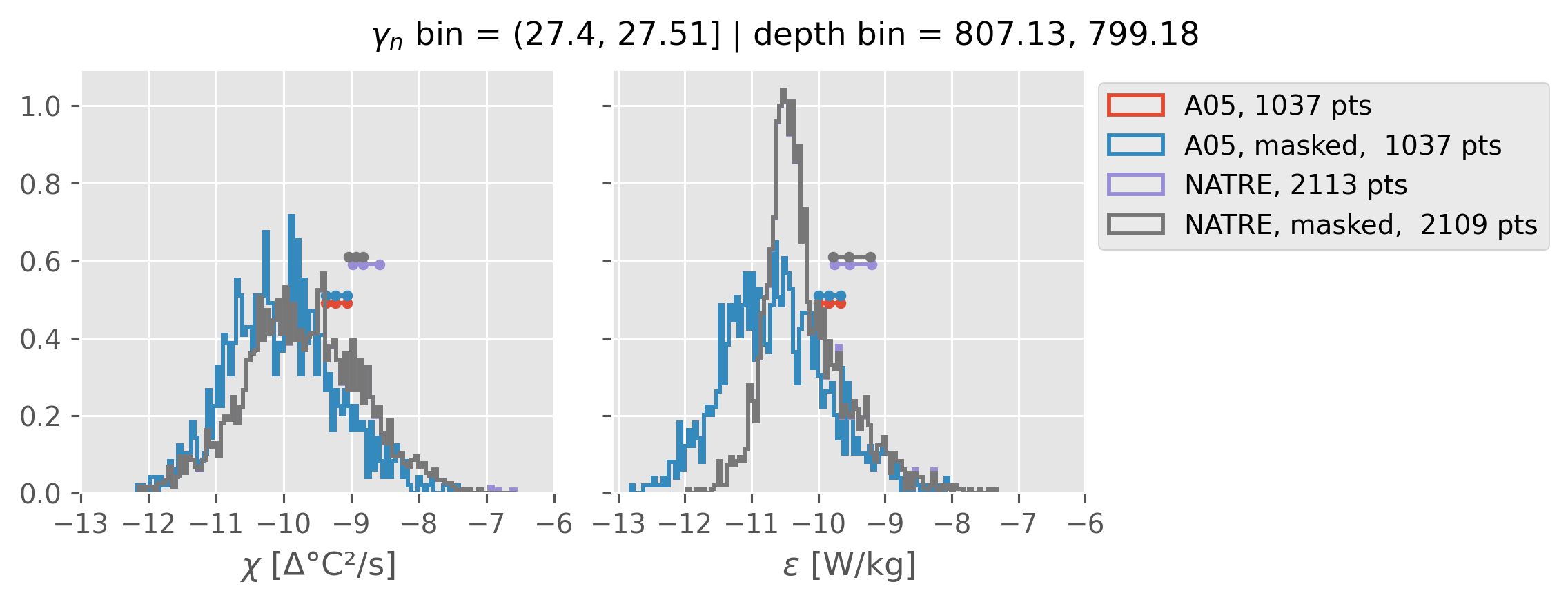
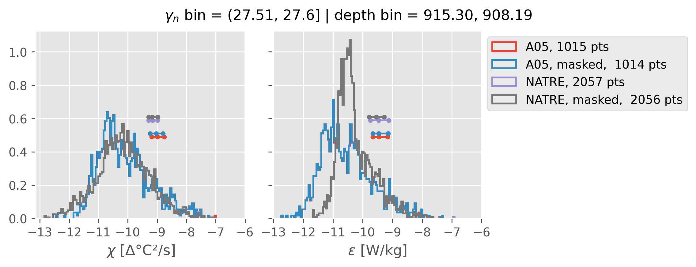
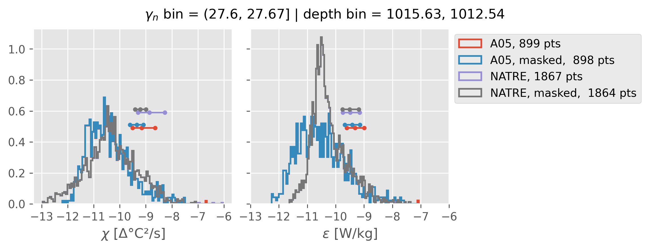
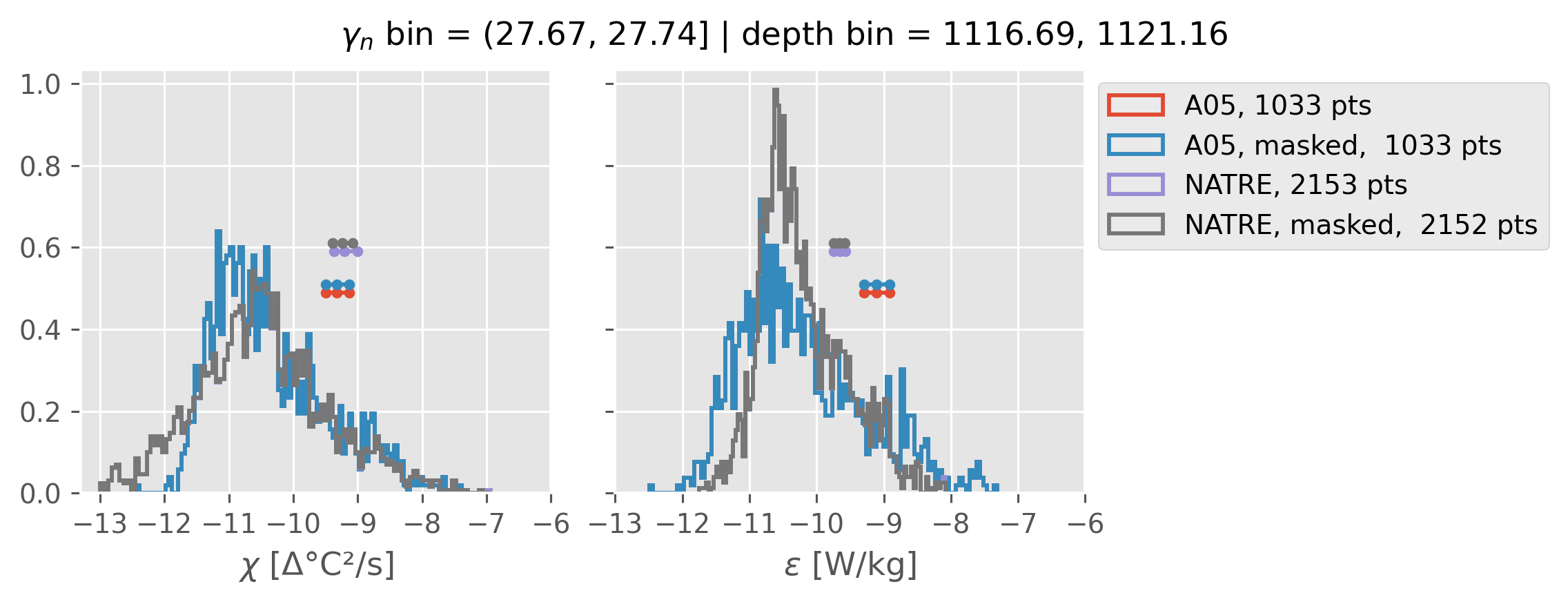
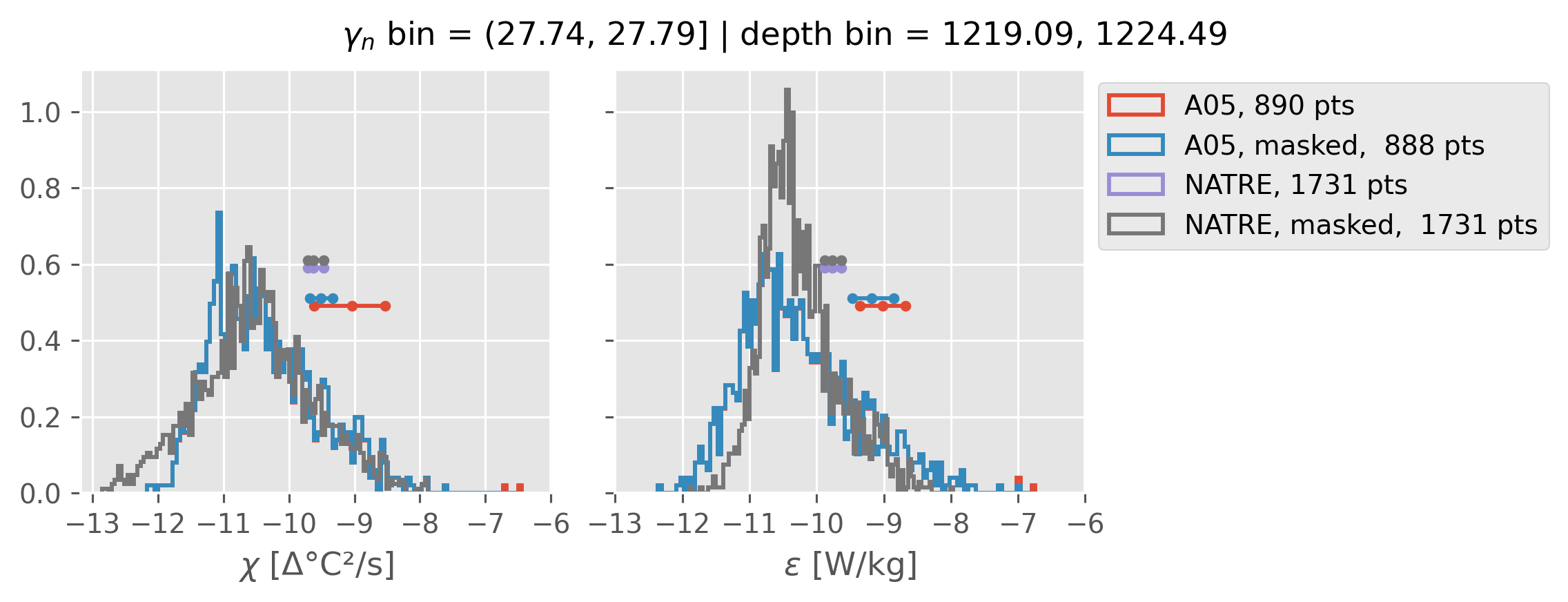
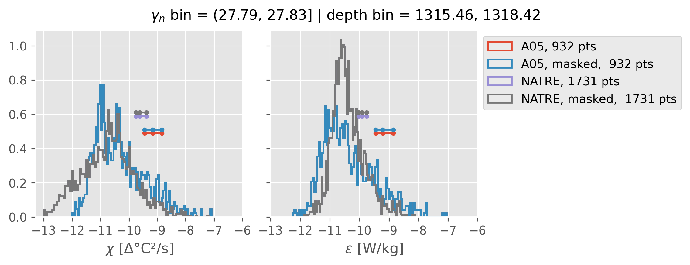
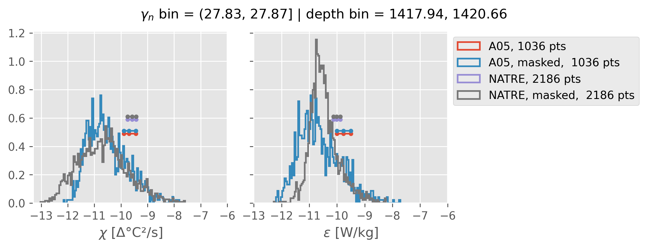
Comparing χ distributions#
These comparisions are using 0.5m NATRE data.
Why is the error so big around 1000m
Error is sensitive to blocksize; I think this is wrong for large blocksize, we don’t get enough independent samples.
NATRE has 5x more points (after coarsening to 2m)
Ignore this following points: I think these high values are cast 131 that is an outlier in T, S too.
but masking out a few high values really reduces error in A05
The high value criterion depends on depth (by comparing with NATRE)
at 1300-ish m we need to throw out χ > 1e-7 (approx.)
at 900-ish m we need to throw out χ > 1e-6 (approx).
A05 looks quite good compared to NATRE at 24.7°N for χ anyway, ε looks hopeless.
Looks like the NATRE data sampled a few different regimes possibly?
And what A05 sampled is plausibly similar to what NATRE sampled at 24.7°N?
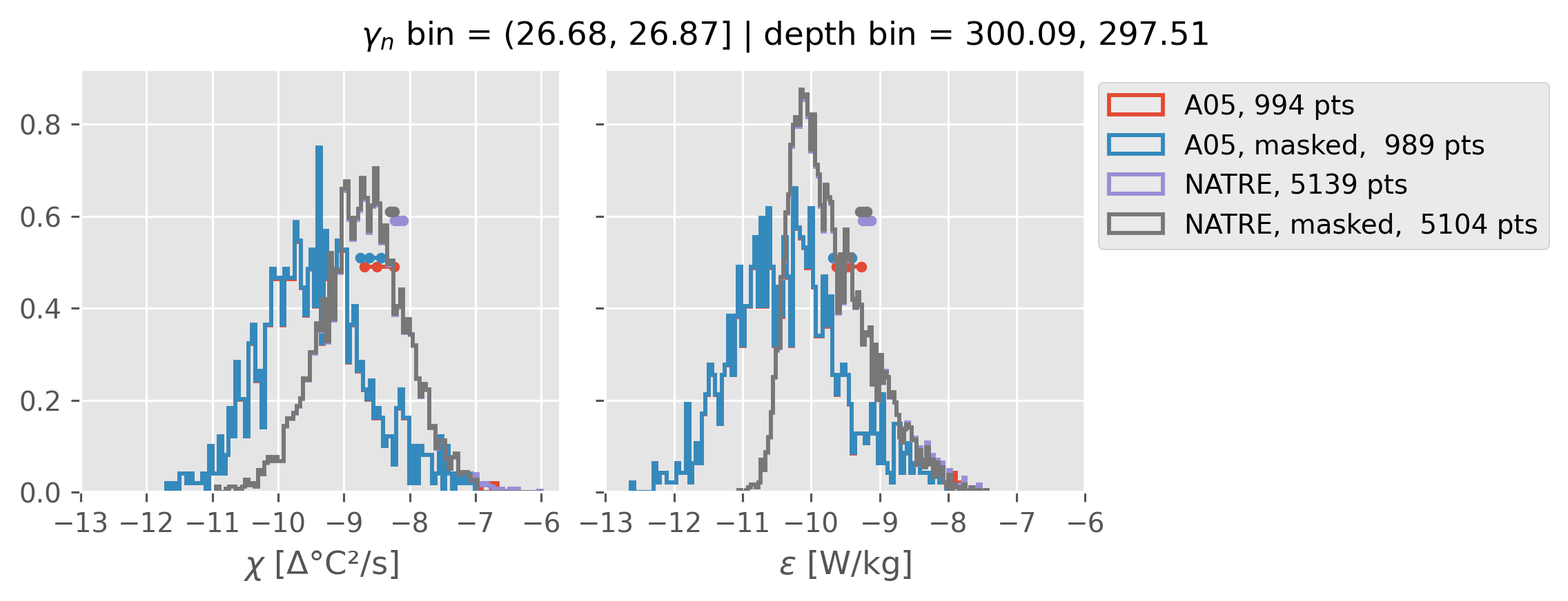
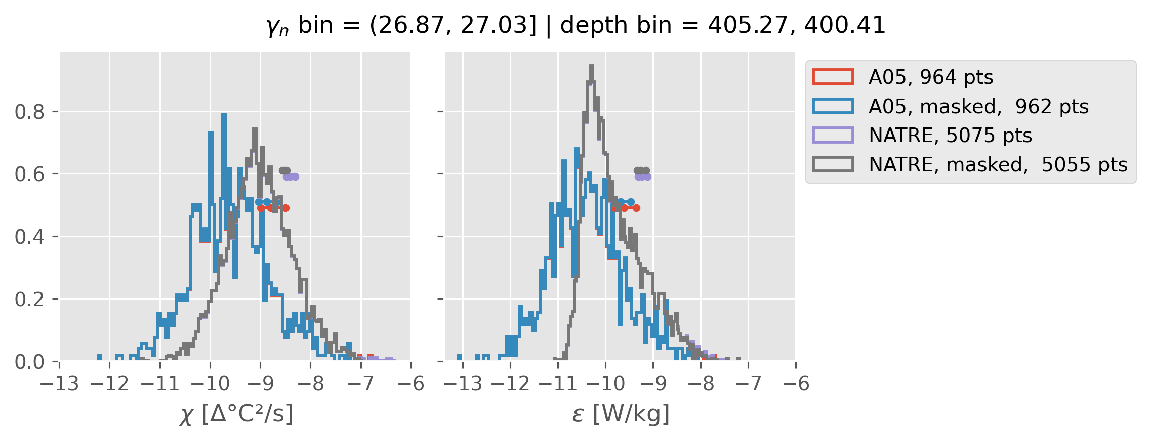
All 2m NATRE data#
inds = slice(0, 14)
print(f"depth range: {np.arange(150, 3150, 100)[inds]}")
print(f"density bins: {bins[inds]}")
a05_grouped = a05.sel(cast=a05_binned.cast).groupby_bins("gamma_n", bins=bins[inds])
natre_grouped = natre_2m.groupby_bins("gamma_n", bins=bins[inds])
ed.natre.compare_chi_distributions(a05_grouped, natre_grouped)
depth range: [ 150 250 350 450 550 650 750 850 950 1050 1150 1250 1350 1450]
density bins: [26.43 26.68 26.87 27.03 27.16 27.28 27.4 27.51 27.6 27.67 27.74 27.79
27.83 27.87]
(26.43, 26.68]
(26.68, 26.87]
(26.87, 27.03]
(27.03, 27.16]
(27.16, 27.28]
(27.28, 27.4]
(27.4, 27.51]
(27.51, 27.6]
(27.6, 27.67]
(27.67, 27.74]
(27.74, 27.79]
(27.79, 27.83]
(27.83, 27.87]
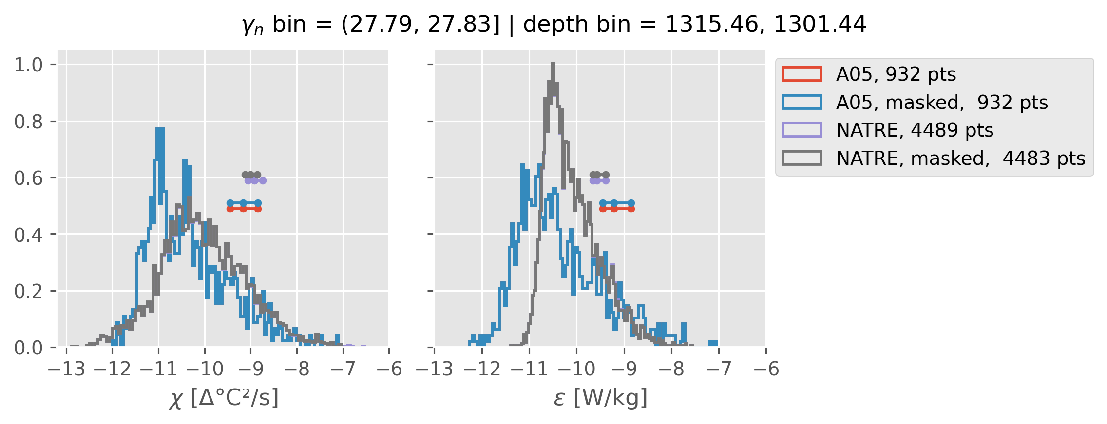
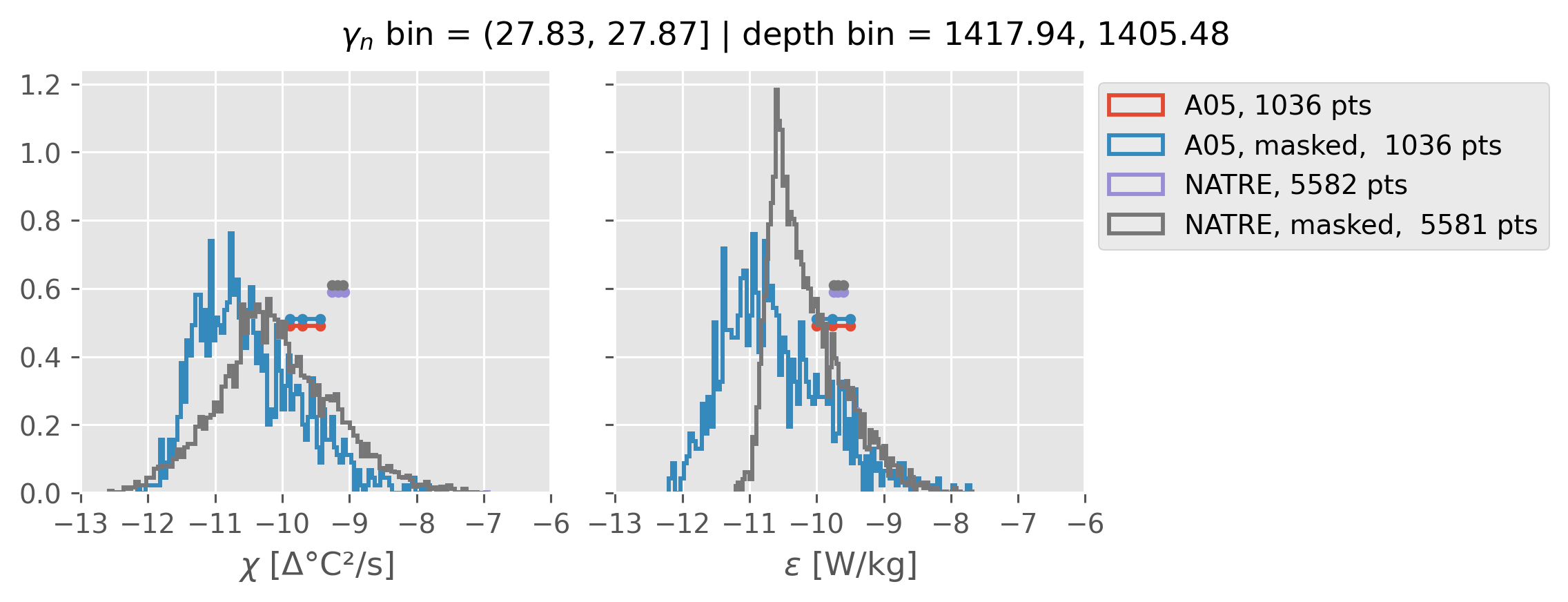
All 0.5m NATRE data#
inds = slice(0, 14)
print(f"depth range: {np.arange(150, 3150, 100)[inds]}")
print(f"density bins: {bins[inds]}")
a05_grouped = a05.sel(cast=a05_binned.cast).groupby_bins("gamma_n", bins=bins[inds])
natre_grouped = natre.groupby_bins("gamma_n", bins=bins[inds])
ed.natre.compare_chi_distributions(a05_grouped, natre_grouped)
depth range: [ 150 250 350 450 550 650 750 850 950 1050 1150 1250 1350 1450]
density bins: [26.43 26.68 26.87 27.03 27.16 27.28 27.4 27.51 27.6 27.67 27.74 27.79
27.83 27.87]
(26.43, 26.68]
(26.68, 26.87]
(26.87, 27.03]
(27.03, 27.16]
(27.16, 27.28]
(27.28, 27.4]
(27.4, 27.51]
(27.51, 27.6]
(27.6, 27.67]
(27.67, 27.74]
(27.74, 27.79]
(27.79, 27.83]
(27.83, 27.87]
2m NATRE at 24.7°N#
inds = slice(0, 14)
print(f"depth range: {np.arange(150, 3150, 100)[inds]}")
print(f"density bins: {bins[inds]}")
a05_grouped = a05.sel(cast=a05_binned.cast).groupby_bins("gamma_n", bins=bins[inds])
natre_grouped = natre_2m.sel(latitude=24.7, method="nearest").groupby_bins(
"gamma_n", bins=bins[inds]
)
ed.natre.compare_chi_distributions(a05_grouped, natre_grouped)
depth range: [ 150 250 350 450 550 650 750 850 950 1050 1150 1250 1350 1450]
density bins: [26.43 26.68 26.87 27.03 27.16 27.28 27.4 27.51 27.6 27.67 27.74 27.79
27.83 27.87]
(26.43, 26.68]
(26.68, 26.87]
(26.87, 27.03]
(27.03, 27.16]
(27.16, 27.28]
(27.28, 27.4]
(27.4, 27.51]
(27.51, 27.6]
(27.6, 27.67]
(27.67, 27.74]
(27.74, 27.79]
(27.79, 27.83]
(27.83, 27.87]
0.5m NATRE at 24.7°N#
inds = slice(0, 14)
print(f"depth range: {np.arange(150, 3150, 100)[inds]}")
print(f"density bins: {bins[inds]}")
a05_grouped = a05.sel(cast=a05_binned.cast).groupby_bins("gamma_n", bins=bins[inds])
natre_grouped = natre.sel(latitude=24.7, method="nearest").groupby_bins(
"gamma_n", bins=bins[inds]
)
ed.natre.compare_chi_distributions(a05_grouped, natre_grouped)
depth range: [ 150 250 350 450 550 650 750 850 950 1050 1150 1250 1350 1450]
density bins: [26.43 26.68 26.87 27.03 27.16 27.28 27.4 27.51 27.6 27.67 27.74 27.79
27.83 27.87]
(26.43, 26.68]
(26.68, 26.87]
(26.87, 27.03]
(27.03, 27.16]
(27.16, 27.28]
(27.28, 27.4]
(27.4, 27.51]
(27.51, 27.6]
(27.6, 27.67]
(27.67, 27.74]
(27.74, 27.79]
(27.79, 27.83]
(27.83, 27.87]
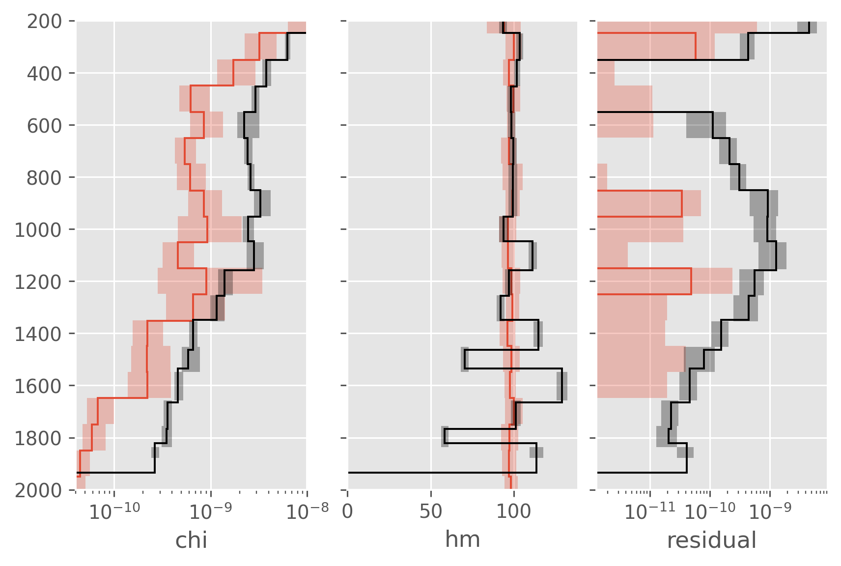
Comparing some terms#
f, ax = plt.subplots(1, 3, sharey=True, constrained_layout=True)
for var, axx in zip(["chi", "hm", "residual"], ax.flat):
dcpy.plots.fill_between_bounds(a05_binned, var, y="pres", ax=axx)
dcpy.plots.fill_between_bounds(natre_binned, var, y="pres", color="k", ax=axx)
axx.set_ylim((2000, 200))
axx.set_xlabel(var)
ax[0].set_xscale("log")
ax[0].set_xlim([4e-11, 1e-8])
ax[2].set_xscale("log")
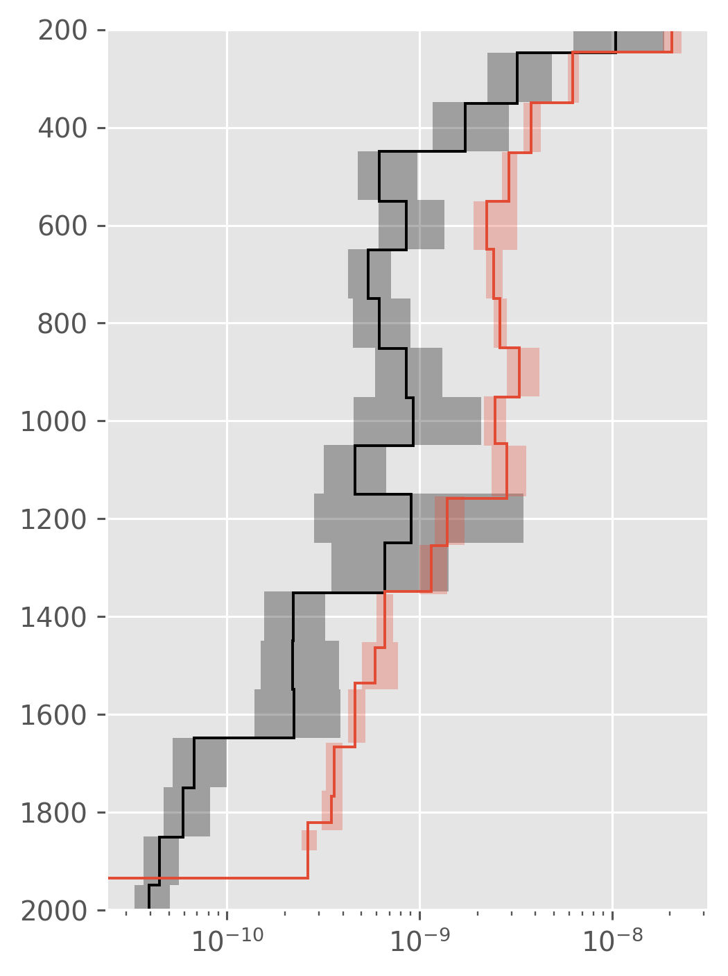
dcpy.plots.fill_between_bounds(a05_binned, "chi", y="pres", color="k")
dcpy.plots.fill_between_bounds(natre_binned, "chi", y="pres")
plt.ylim((2000, 200))
plt.xscale("log")
plt.gcf().set_size_inches((4, 6))
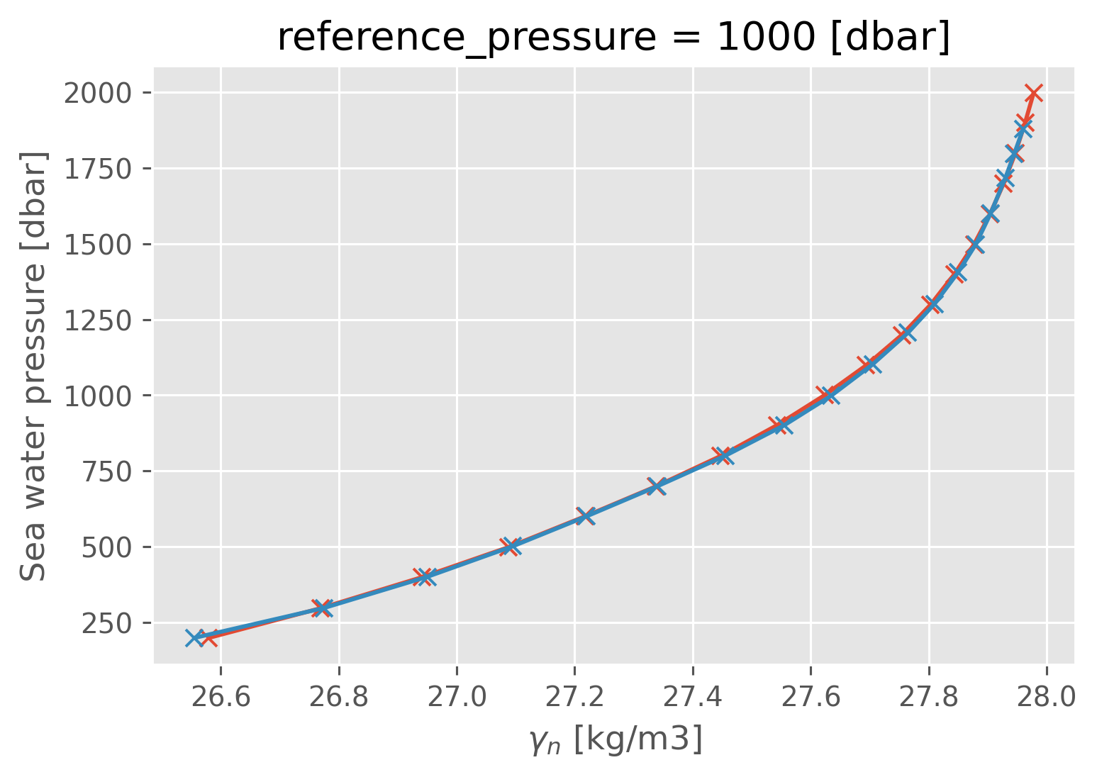
a05_binned.gamma_n.plot(y="pres", marker="x")
natre_binned.gamma_n.plot(y="pres", marker="x")
[<matplotlib.lines.Line2D at 0x181932070>]
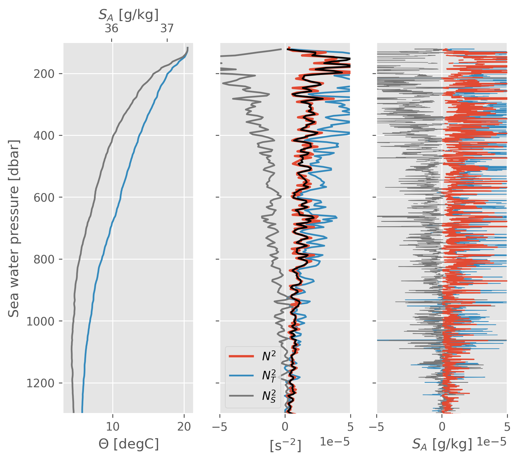
Finestructure metrics#
There is compensated T-S variability at all levels really. The question is what is dominant.
Why is the top 500m different from 1000-ish m?
There is compensated variability at all levels really.
I think this is why we need to care about lateral gradients of stuff…
Perhaps it’s enhanced \(N_T^2/N^2\) at levels where the mean lateral spice gradient is large
from functools import partial
import xrft
import gsw
profile = a05.sel(cast=136)
profile = natre.isel(latitude=9, longitude=6) # .drop_vars("depth", erro)
Z = profile.SA.cf["Z"]
Zname = Z.name
profile["NT2"] = (
-9.81
* gsw.alpha(profile.SA, profile.CT, Z)
* profile.CT.cf.interpolate_na("Z").cf.differentiate("Z")
)
profile["NS2"] = (
9.81
* gsw.beta(profile.SA, profile.CT, Z)
* profile.SA.cf.interpolate_na("Z").cf.differentiate("Z")
)
smoothed = (
profile.cf.rolling(Z=10, center=True, min_periods=1)
.mean()
.cf.coarsen(Z=10, boundary="trim")
.mean()
)
smoothed["NT2"] = (
-9.81
* gsw.alpha(smoothed.SA, smoothed.CT, smoothed[Zname])
* smoothed.CT.cf.interpolate_na("Z").cf.differentiate("Z")
)
smoothed["NS2"] = (
9.81
* gsw.beta(smoothed.SA, smoothed.CT, smoothed[Zname])
* smoothed.SA.cf.interpolate_na("Z").cf.differentiate("Z")
)
f, ax = plt.subplots(1, 3, sharey=True)
smoothed.CT.cf.plot(ax=ax[0], color="C1")
axS = ax[0].twiny()
axS.grid(False)
smoothed.SA.cf.plot(color="C3", ax=axS)
smoothed.N2.cf.plot(lw=2, zorder=5, ax=ax[1])
smoothed.NT2.cf.plot(ax=ax[1])
smoothed.NS2.cf.plot(color="C3", ax=ax[1])
(smoothed.NT2 + smoothed.NS2).cf.plot(color="k", ax=ax[1], zorder=8)
ax[1].set_xlim([-5e-5, 5e-5])
ax[1].legend(["$N^2$", "$N_T^2$", "$N_S^2$"])
profile.N2.cf.plot(lw=1, zorder=5, ax=ax[2])
profile.NT2.cf.plot(ax=ax[2], lw=0.5)
profile.NS2.cf.plot(color="C3", ax=ax[2], lw=0.5)
ax[2].set_xlim([-5e-5, 5e-5])
# ax[2].legend(["$N^2$", "$N_T^2$", "$N_S^2$"])
dcpy.plots.clean_axes(ax)
[aa.set_title("") for aa in ax]
axS.set_title("")
ax[1].set_xlabel("[s$^{-2}$]")
ax[1].set_ylim((1300, 100))
f.set_size_inches((7, 6))
natre["NT2"] = (
-9.81
* gsw.alpha(natre.SA, natre.CT, Z)
* natre.CT.cf.interpolate_na("Z").cf.differentiate("Z")
)
natre["NS2"] = (
9.81
* gsw.beta(natre.SA, natre.CT, Z)
* natre.SA.cf.interpolate_na("Z").cf.differentiate("Z")
)
windows = (
natre[["NT2", "NS2", "N2"]]
.sel(pres=slice(2000))
.interpolate_na("pres")
.rolling(pres=128 * 2, center=True)
.construct({"pres": "window"}, stride=128)
)
windows["window"] = np.arange(0, 128, 0.5)
spec = (
windows.map(
partial(
xrft.power_spectrum,
dim="window",
real_dim="window",
window="hann",
window_correction=True,
)
)
.isel(freq_window=slice(1, None))
.coarsen(freq_window=3, boundary="trim")
.mean()
)
spec
<xarray.Dataset>
Dimensions: (latitude: 10, longitude: 10, pres: 32, freq_window: 42)
Coordinates:
* pres (pres) float64 10.0 74.0 138.0 ... 1.866e+03 1.93e+03 1.994e+03
* latitude (latitude) float64 27.5 27.1 26.7 26.3 ... 25.1 24.7 24.3 23.9
* longitude (longitude) float64 -30.7 -30.3 -29.8 ... -27.6 -27.2 -26.8
time (latitude, longitude) datetime64[ns] 1992-03-28T15:28:59.999...
* freq_window (freq_window) float64 0.01562 0.03906 0.0625 ... 0.9531 0.9766
Data variables:
NT2 (latitude, longitude, pres, freq_window) float64 nan ... nan
NS2 (latitude, longitude, pres, freq_window) float64 nan ... nan
N2 (latitude, longitude, pres, freq_window) float64 nan ... nan
Attributes: (12/13)
Conventions: CF-1.6
netcdf_version: 4
project: North Atlantic Tracer Release Experiment (NATRE)
expocode: 32OC250_4
cast_number: 3.0
title: Microstructure profiler data from the ship Oceanus...
... ...
latitude: 27.533166666666666
longitude: -30.723333333333333
chief_scientist: Raymond W. Schmitt
data_originator: Polzin
institution: WHOI
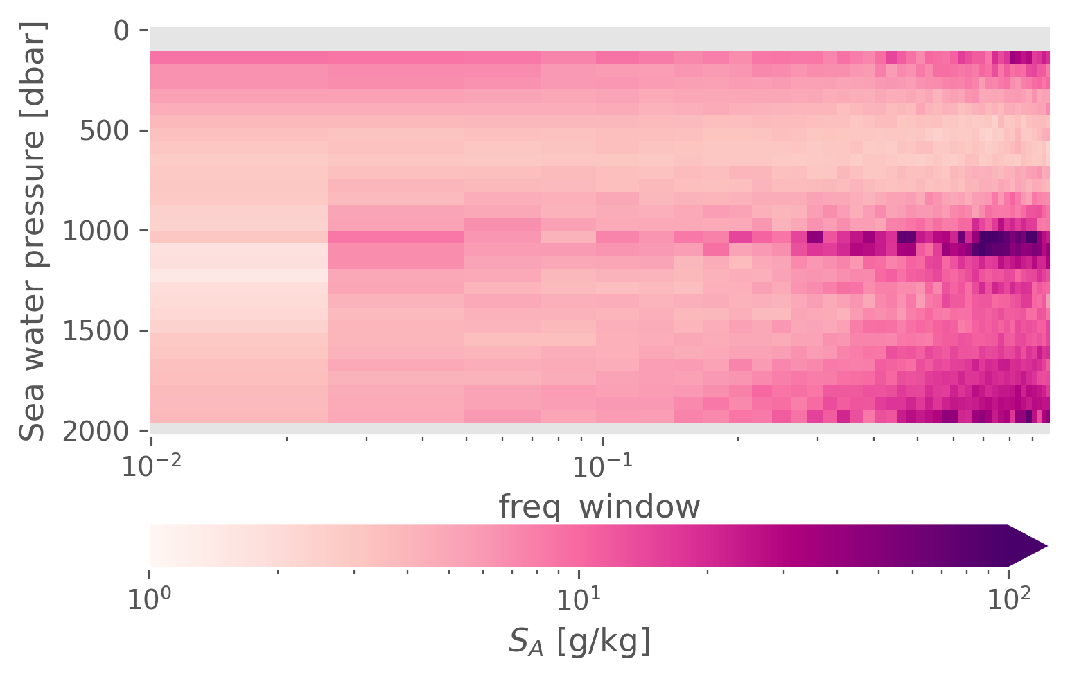
data_assembly_center: CCHDOmeanspec = spec.mean(["latitude", "longitude"])
(meanspec.NT2 / meanspec.N2).cf.plot(
# row="variable",
cbar_kwargs={"orientation": "horizontal"},
xscale="log",
norm=mpl.colors.LogNorm(1, 1e2),
# center=10,
cmap=mpl.cm.RdPu,
)
<matplotlib.collections.QuadMesh at 0x18c3d4c70>
meanspec = spec.mean(["longitude"])
(meanspec.NT2 / meanspec.N2).sortby("latitude").cf.plot(
col="latitude",
col_wrap=5,
# cbar_kwargs=dcpy.plots.HORCBAR,
xscale="log",
norm=mpl.colors.LogNorm(1, 50),
# center=10,
cmap=mpl.cm.RdPu,
)
<xarray.plot.facetgrid.FacetGrid at 0x18c4dacd0>
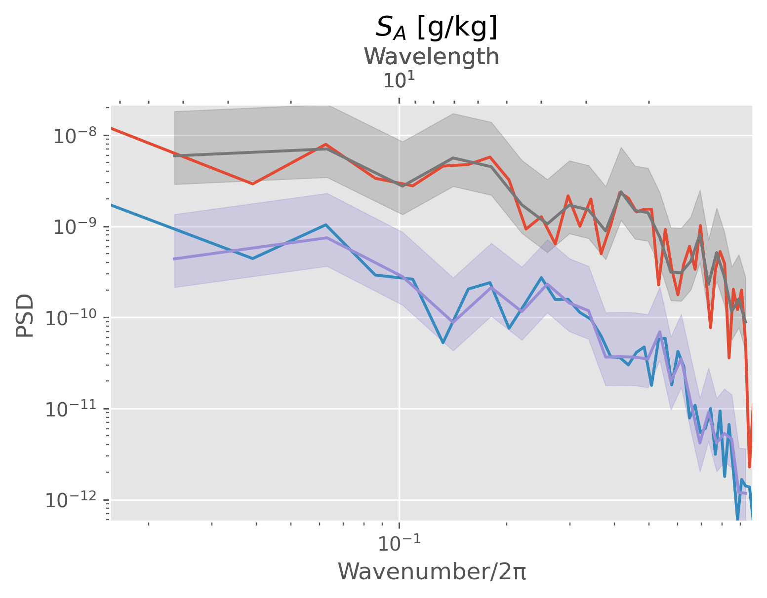
P = 1000
spec.NT2.sel(pres=P, method="nearest").plot()
spec.N2.sel(pres=P, method="nearest").plot(xscale="log", yscale="log")
dcpy.ts.PlotSpectrum(
windows.sel(pres=P, method="nearest").N2, ax=plt.gca(), multitaper=False
)
dcpy.ts.PlotSpectrum(
windows.sel(pres=P, method="nearest").NT2, ax=plt.gca(), multitaper=False
)
([<matplotlib.lines.Line2D at 0x186785910>],
<AxesSubplot:title={'center':' $S_A$ [g/kg]'}, xlabel='Wavenumber/2π', ylabel='PSD'>)