EQUIX#
import cf_xarray
import dcpy
import distributed
import hvplot.xarray
import matplotlib as mpl
import matplotlib.pyplot as plt
import numpy as np
import pandas as pd
import pump
import xgcm
from dcpy.oceans import read_osu_microstructure_mat
from IPython.display import Image
from scipy.io import loadmat

import eddydiff
import eddydiff as ed
import xarray as xr

xr.set_options(keep_attrs=True)

plt.rcParams["figure.dpi"] = 140
plt.rcParams["savefig.dpi"] = 200
plt.style.use("ggplot")
Todo#
[x] See if IOP variance terms match chameleon
[x] is there a consolidated TAO data file
[x] are they in the PMEL TAO files?
[ ] use 10 min averages to calculate KT, Jq
[ ] What is happening with the top few bins
[x] Take out Chameleon MLD properly not just slice it out
[x] filter χpod bad estimates using dT/dz - already done
[x] filter out binned estimates using count
[ ] pick bins that don’t outcrop?
[ ] try chameleon dTdz using xgcm transform
[ ] look at T-S diagram north, south of the equator
Data file notes#
indus/chipod/eq08_long/processed/chi_analysis/deglitched/
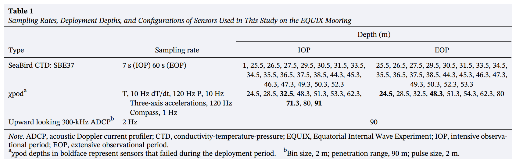
allchi_eq08_long.matEQUIX EOP APL mooring; renamed toequix_eop.matmean_chi_*.matseem to be IOP files per χpod
EOP units: 204 205 304 312 314 315 328
mean_chi vs summary files
summary files: T1, T2, AZ etc.
mean_chi files: T1, T2, eps, chi, KT, Jq
Image("../images/equix-chipods.png")
Image("../images/equix-tao-chipods.png")
Chameleon#
chameleon = xr.open_dataset("/home/deepak/datasets/microstructure/osu/equix.nc")
del chameleon["dTdz"]  # not potential temperature?
chameleon = ed.sections.add_ancillary_variables(chameleon)
# take out ML
chameleon = chameleon.where(chameleon.depth > chameleon.mld)
chameleon = chameleon.cf.set_coords(["latitude", "longitude"])
bins = ed.sections.choose_bins(
    chameleon.cf["neutral_density"], depth_range=np.arange(20, 200, 15)
)

chameleon
<xarray.Dataset>
Dimensions:      (depth: 200, time: 2624, zeuc: 80)
Coordinates:
  * depth        (depth) uint64 1 2 3 4 5 6 7 8 ... 194 195 196 197 198 199 200
    lon          (time) float64 -139.9 -139.9 -139.9 ... -139.9 -139.9 -139.9
    lat          (time) float64 0.06246 0.0622 0.06263 ... 0.06317 0.06341
  * time         (time) datetime64[ns] 2008-10-24T20:36:23 ... 2008-11-08T19:...
  * zeuc         (zeuc) float64 -200.0 -195.0 -190.0 ... 185.0 190.0 195.0
Data variables: (12/46)
    pmax         (time, depth) float64 nan nan 205.9 205.9 ... 203.9 203.9 203.9
    castnumber   (time, depth) float64 nan nan 16.0 ... 2.668e+03 2.668e+03
    AX_TILT      (depth, time) float64 nan nan nan nan ... 0.7031 4.232 1.28
    AY_TILT      (depth, time) float64 nan nan nan nan ... -2.623 -2.121 0.05032
    AZ2          (depth, time) float64 nan nan nan ... 2.612e-06 3.208e-06
    C            (depth, time) float64 nan nan nan nan ... 4.135 4.137 4.164
    ...           ...
    chi_masked   (depth, time) float64 nan nan nan ... 4e-09 2.592e-09 9.245e-09
    Krho         (depth, time) float64 nan nan nan ... 2.642e-05 9.09e-06
    KrhoTz       (depth, time) float64 nan nan nan ... 2.195e-06 4.328e-07
    eps_chi      (depth, time) float64 nan nan nan ... 4.389e-11 5.913e-10
    Kt           (depth, time) float64 nan nan nan ... 1.877e-07 2.039e-06
    KtTz         (depth, time) float64 nan nan nan ... 1.559e-08 9.708e-08
Attributes:
    starttime:  ['Time:20:34:29 298   ' 'Time:20:42:18 298   ' 'Time:20:52:14...
    endtime:    ['Time:20:38:29 298   ' 'Time:20:46:29 298   ' 'Time:20:56:29...
name: EQUIX- depth: 200
- time: 2624
- zeuc: 80
- depth(depth)uint641 2 3 4 5 6 ... 196 197 198 199 200
- positive :
- down
- axis :
- Z
array([ 1, 2, 3, 4, 5, 6, 7, 8, 9, 10, 11, 12, 13, 14, 15, 16, 17, 18, 19, 20, 21, 22, 23, 24, 25, 26, 27, 28, 29, 30, 31, 32, 33, 34, 35, 36, 37, 38, 39, 40, 41, 42, 43, 44, 45, 46, 47, 48, 49, 50, 51, 52, 53, 54, 55, 56, 57, 58, 59, 60, 61, 62, 63, 64, 65, 66, 67, 68, 69, 70, 71, 72, 73, 74, 75, 76, 77, 78, 79, 80, 81, 82, 83, 84, 85, 86, 87, 88, 89, 90, 91, 92, 93, 94, 95, 96, 97, 98, 99, 100, 101, 102, 103, 104, 105, 106, 107, 108, 109, 110, 111, 112, 113, 114, 115, 116, 117, 118, 119, 120, 121, 122, 123, 124, 125, 126, 127, 128, 129, 130, 131, 132, 133, 134, 135, 136, 137, 138, 139, 140, 141, 142, 143, 144, 145, 146, 147, 148, 149, 150, 151, 152, 153, 154, 155, 156, 157, 158, 159, 160, 161, 162, 163, 164, 165, 166, 167, 168, 169, 170, 171, 172, 173, 174, 175, 176, 177, 178, 179, 180, 181, 182, 183, 184, 185, 186, 187, 188, 189, 190, 191, 192, 193, 194, 195, 196, 197, 198, 199, 200], dtype=uint64) - lon(time)float64-139.9 -139.9 ... -139.9 -139.9
- standard_name :
- longitude
- units :
- degrees_east
array([-139.868406 , -139.86840867, -139.86840817, ..., -139.87721183, -139.87707 , -139.877121 ]) - lat(time)float640.06246 0.0622 ... 0.06317 0.06341
- standard_name :
- latitude
- units :
- degrees_north
array([0.06245817, 0.06219917, 0.06263083, ..., 0.06311433, 0.063169 , 0.0634125 ]) - time(time)datetime64[ns]2008-10-24T20:36:23 ... 2008-11-...
array(['2008-10-24T20:36:23.000000000', '2008-10-24T20:44:18.000000000', '2008-10-24T20:54:17.000000000', ..., '2008-11-08T18:58:49.000000000', '2008-11-08T19:06:14.000000000', '2008-11-08T19:13:47.000000000'], dtype='datetime64[ns]') - zeuc(zeuc)float64-200.0 -195.0 ... 190.0 195.0
- positive :
- up
- axis :
- Z
- long_name :
- $z - z_{EUC}$
- units :
- m
array([-200., -195., -190., -185., -180., -175., -170., -165., -160., -155.,
       -150., -145., -140., -135., -130., -125., -120., -115., -110., -105.,
       -100.,  -95.,  -90.,  -85.,  -80.,  -75.,  -70.,  -65.,  -60.,  -55.,
        -50.,  -45.,  -40.,  -35.,  -30.,  -25.,  -20.,  -15.,  -10.,   -5.,
          0.,    5.,   10.,   15.,   20.,   25.,   30.,   35.,   40.,   45.,
         50.,   55.,   60.,   65.,   70.,   75.,   80.,   85.,   90.,   95.,
        100.,  105.,  110.,  115.,  120.,  125.,  130.,  135.,  140.,  145.,
        150.,  155.,  160.,  165.,  170.,  175.,  180.,  185.,  190.,  195.])
- pmax(time, depth)float64nan nan 205.9 ... 203.9 203.9 203.9
array([[ nan, nan, 205.93651536, ..., 205.93651536, 205.93651536, 205.93651536], [ nan, nan, nan, ..., 199.00510569, 199.00510569, 199.00510569], [ nan, nan, nan, ..., 202.00242137, 202.00242137, 202.00242137], ..., [ nan, nan, nan, ..., 202.01574447, 202.01574447, 202.01574447], [ nan, nan, nan, ..., 221.05402492, 221.05402492, 221.05402492], [ nan, nan, nan, ..., 203.86125274, 203.86125274, 203.86125274]]) - castnumber(time, depth)float64nan nan ... 2.668e+03 2.668e+03
array([[ nan, nan, 16., ..., 16., 16., 16.], [ nan, nan, nan, ..., 17., 17., 17.], [ nan, nan, nan, ..., 18., 18., 18.], ..., [ nan, nan, nan, ..., 2666., 2666., 2666.], [ nan, nan, nan, ..., 2667., 2667., 2667.], [ nan, nan, nan, ..., 2668., 2668., 2668.]]) - AX_TILT(depth, time)float64nan nan nan ... 0.7031 4.232 1.28
array([[ nan, nan, nan, ..., nan, nan, nan], [ nan, nan, nan, ..., nan, nan, nan], [-0.13846664, nan, nan, ..., nan, nan, nan], ..., [-0.3999788 , 0.07714795, 0.58404001, ..., 0.49822554, 3.94440538, 0.89481111], [-0.46398325, 0.14535449, 0.63026535, ..., 0.77353237, 3.86853844, 1.1196056 ], [-0.37911422, nan, 0.66167671, ..., 0.70312844, 4.23175887, 1.27969235]]) - AY_TILT(depth, time)float64nan nan nan ... -2.121 0.05032
array([[ nan, nan, nan, ..., nan, nan, nan], [ nan, nan, nan, ..., nan, nan, nan], [ 4.21619137, nan, nan, ..., nan, nan, nan], ..., [-1.98386615, -1.61662696, -1.81510711, ..., -3.30561771, -1.87552638, -0.13780247], [-1.63654255, -1.54284209, -0.53946635, ..., -2.81611526, -1.96872885, 0.09218141], [-1.76751644, nan, -1.11048116, ..., -2.62284326, -2.12143302, 0.05032124]]) - AZ2(depth, time)float64nan nan nan ... 2.612e-06 3.208e-06
array([[ nan, nan, nan, ..., nan, nan, nan], [ nan, nan, nan, ..., nan, nan, nan], [1.87232177e-04, nan, nan, ..., nan, nan, nan], ..., [6.75551720e-06, 4.57687418e-06, 5.43906674e-06, ..., 1.50305291e-05, 2.90585558e-06, 4.50582475e-06], [1.17132603e-05, 5.66169186e-06, 1.36095944e-05, ..., 2.24203923e-06, 2.69464518e-06, 5.84454101e-06], [8.83178862e-06, nan, 6.95564234e-06, ..., 2.91223680e-06, 2.61247030e-06, 3.20761422e-06]]) - C(depth, time)float64nan nan nan ... 4.135 4.137 4.164
array([[ nan, nan, nan, ..., nan, nan, nan], [ nan, nan, nan, ..., nan, nan, nan], [5.25770276, nan, nan, ..., nan, nan, nan], ..., [4.15348212, 4.1562709 , 4.15720205, ..., 4.14974132, 4.14999048, 4.17485331], [4.15389983, 4.15688293, 4.15742006, ..., 4.14276969, 4.14630483, 4.16952148], [4.15413389, nan, 4.15719298, ..., 4.13482505, 4.13726266, 4.16428369]]) - chi(depth, time)float64nan nan nan ... 2.592e-09 9.245e-09
- long_name :
- $χ$
- units :
- °C²/s
array([[ nan, nan, nan, ..., nan, nan, nan], [ nan, nan, nan, ..., nan, nan, nan], [5.42809819e-07, nan, nan, ..., nan, nan, nan], ..., [1.17618518e-11, 1.51284284e-11, 1.55842645e-10, ..., 1.00900275e-07, 6.94714665e-07, 7.72806894e-09], [1.32466080e-11, 4.03601274e-11, 1.91113796e-11, ..., 2.34244678e-07, 2.62691364e-06, 7.94421817e-09], [2.13465286e-11, nan, 1.42169165e-11, ..., 4.00016873e-09, 2.59171599e-09, 9.24455507e-09]]) - DRHODZ(depth, time)float64nan nan nan ... 0.004887 0.00606
array([[ nan, nan, nan, ..., nan, nan, nan], [ nan, nan, nan, ..., nan, nan, nan], [0.01732687, nan, nan, ..., nan, nan, nan], ..., [0.00159717, 0.00099967, 0.00072395, ..., 0.00777257, 0.00572349, 0.00708041], [0.00145471, 0.0007196 , 0.00086594, ..., 0.00934785, 0.0087413 , 0.00623388], [0.0015311 , nan, 0.00063949, ..., 0.00626084, 0.00488731, 0.00605951]]) - eps(depth, time)float64nan nan nan ... 6.178e-09 2.636e-09
- long_name :
- $ε$
- units :
- W/kg
array([[ nan, nan, nan, ..., nan, nan, nan], [ nan, nan, nan, ..., nan, nan, nan], [ nan, nan, nan, ..., nan, nan, nan], ..., [6.96240408e-10, 2.39643180e-09, 1.27925802e-09, ..., 2.97011866e-08, nan, 5.30762709e-09], [3.22168218e-10, 8.85430965e-10, 1.54639088e-09, ..., 6.88137519e-09, 1.26222122e-07, nan], [ nan, nan, 3.55171006e-09, ..., 3.13672119e-09, 6.17819337e-09, 2.63627225e-09]]) - EPSILON1(depth, time)float64nan nan nan ... 6.572e-09 4.344e-09
array([[ nan, nan, nan, ..., nan, nan, nan], [ nan, nan, nan, ..., nan, nan, nan], [ nan, nan, nan, ..., nan, nan, nan], ..., [6.96240408e-10, 7.80493785e-10, 1.27925802e-09, ..., 3.49214176e-08, nan, 7.25170224e-09], [3.22168218e-10, 8.85430965e-10, 1.54639088e-09, ..., 9.77033274e-09, 1.53937468e-07, nan], [ nan, nan, 3.55171006e-09, ..., 2.47166751e-09, 6.57190476e-09, 4.34368847e-09]]) - EPSILON2(depth, time)float64nan nan nan ... 5.784e-09 9.289e-10
array([[ nan, nan, nan, ..., nan, nan, nan], [ nan, nan, nan, ..., nan, nan, nan], [ nan, nan, nan, ..., nan, nan, nan], ..., [8.66262735e-09, 4.01236982e-09, 7.69519866e-09, ..., 2.44809556e-08, nan, 3.36355195e-09], [2.55864584e-08, 8.16851488e-09, 2.76931354e-07, ..., 3.99241764e-09, 9.85067754e-08, nan], [ nan, nan, 3.34671328e-08, ..., 3.80177488e-09, 5.78448199e-09, 9.28856029e-10]]) - FALLSPD(depth, time)float64nan nan nan ... 73.68 74.23 73.72
array([[ nan, nan, nan, ..., nan, nan, nan], [ nan, nan, nan, ..., nan, nan, nan], [117.01893601, nan, nan, ..., nan, nan, nan], ..., [ 70.66059168, 68.89335476, 68.35594549, ..., 73.36311557, 76.37039051, 72.15674015], [ 66.0835682 , 68.5683379 , 57.51229511, ..., 73.68654834, 75.78505871, 72.75590847], [ 69.5408982 , nan, 64.9369635 , ..., 73.68007403, 74.23266601, 73.72112265]]) - MHT(depth, time)float64nan nan nan ... 13.36 13.39 13.63
array([[ nan, nan, nan, ..., nan, nan, nan], [ nan, nan, nan, ..., nan, nan, nan], [24.4569863 , nan, nan, ..., nan, nan, nan], ..., [13.50062455, 13.50232187, 13.51214501, ..., 13.49363389, 13.49803401, 13.7219205 ], [13.50205545, 13.50582842, 13.51252495, ..., 13.43453994, 13.46303391, 13.67271452], [13.50169137, nan, 13.50961328, ..., 13.36115077, 13.38807874, 13.62652538]]) - N2(depth, time)float64nan nan nan ... 4.678e-05 5.801e-05
- long_name :
- $N²$
array([[ nan, nan, nan, ..., nan, nan, nan], [ nan, nan, nan, ..., nan, nan, nan], [ nan, nan, nan, ..., nan, nan, nan], ..., [1.52843602e-05, 9.56689133e-06, 6.92781248e-06, ..., 7.44032795e-05, 5.47807795e-05, 6.77780203e-05], [1.39210577e-05, 6.88659760e-06, 8.28652498e-06, ..., 8.94827089e-05, 8.36648197e-05, 5.96745392e-05], [1.46520449e-05, nan, 6.11957220e-06, ..., 5.99322176e-05, 4.67774482e-05, 5.80053170e-05]]) - pres(depth, time)float64nan nan nan ... 200.0 200.0 200.0
- standard_name :
- sea_water_pressure
- units :
- dbar
array([[ nan, nan, nan, ..., nan, nan, nan], [ nan, nan, nan, ..., nan, nan, nan], [ 3.01252786, nan, nan, ..., nan, nan, nan], ..., [198.00265734, 198.0004711 , 197.99984601, ..., 197.99459749, 197.99978955, 198.0015132 ], [199.00301925, 199.00510569, 199.00631631, ..., 199.00448072, 199.00628156, 199.00489772], [199.99484205, nan, 199.99273528, ..., 200.00331355, 199.9988644 , 199.99903749]]) - salt(depth, time)float64nan nan nan ... 34.93 34.93 34.96
- standard_name :
- sea_water_salinity
- units :
- psu
array([[ nan, nan, nan, ..., nan, nan, nan], [ nan, nan, nan, ..., nan, nan, nan], [35.05344093, nan, nan, ..., nan, nan, nan], ..., [34.9961638 , 35.02097547, 35.0206923 , ..., 34.94485747, 34.94327127, 34.96990918], [34.99843771, 35.02305751, 35.0219565 , ..., 34.9378472 , 34.93829672, 34.96477563], [35.00050735, nan, 35.02210145, ..., 34.92858079, 34.92865856, 34.95861769]]) - SCAT(depth, time)float64nan nan nan ... 0.005521 0.005352
array([[ nan, nan, nan, ..., nan, nan, nan], [ nan, nan, nan, ..., nan, nan, nan], [0.03141643, nan, nan, ..., nan, nan, nan], ..., [0.00804034, 0.00829834, 0.0088503 , ..., 0.00658199, 0.0055813 , 0.0061264 ], [0.00886397, 0.0085968 , 0.00859985, ..., 0.00673109, 0.00553154, 0.00584433], [0.00918435, nan, 0.00883484, ..., 0.00619573, 0.00552144, 0.00535185]]) - pden(depth, time)float64nan nan nan ... 26.27 26.26 26.23
- long_name :
- $ρ$
array([[ nan, nan, nan, ..., nan, nan, nan], [ nan, nan, nan, ..., nan, nan, nan], [23.54584534, nan, nan, ..., nan, nan, nan], ..., [26.29388507, 26.31276261, 26.31051514, ..., 26.25056649, 26.24845687, 26.22231475], [26.2953958 , 26.31367257, 26.31144044, ..., 26.25840607, 26.25139929, 26.22865568], [26.29708919, nan, 26.31218545, ..., 26.26601839, 26.26096781, 26.23375296]]) - SIGMA_ORDER(depth, time)float64nan nan nan ... 26.27 26.26 26.23
array([[ nan, nan, nan, ..., nan, nan, nan], [ nan, nan, nan, ..., nan, nan, nan], [23.54579849, nan, nan, ..., nan, nan, nan], ..., [26.29391253, 26.31245867, 26.31066739, ..., 26.25068981, 26.24716886, 26.22187649], [26.29539223, 26.31333338, 26.31141875, ..., 26.26007178, 26.25431434, 26.22811577], [26.29703015, nan, 26.31220693, ..., 26.26697105, 26.26086833, 26.23444197]]) - T(depth, time)float64nan nan nan ... 13.38 13.41 13.65
- standard_name :
- sea_water_temperature
- units :
- celsius
array([[ nan, nan, nan, ..., nan, nan, nan], [ nan, nan, nan, ..., nan, nan, nan], [24.4569863 , nan, nan, ..., nan, nan, nan], ..., [13.50062455, 13.50232187, 13.51214501, ..., 13.51782868, 13.52213554, 13.74865422], [13.50205545, 13.50582842, 13.51252495, ..., 13.45309267, 13.48906756, 13.69895042], [13.50169137, nan, 13.50961328, ..., 13.38095109, 13.40600394, 13.65149054]]) - theta(depth, time)float64nan nan nan ... 13.35 13.38 13.62
- standard_name :
- sea_water_potential_temperature
- units :
- celsius
- long_name :
- $θ$
array([[ nan, nan, nan, ..., nan, nan, nan], [ nan, nan, nan, ..., nan, nan, nan], [24.45619486, nan, nan, ..., nan, nan, nan], ..., [13.47251088, 13.47410045, 13.48396391, ..., 13.49006132, 13.4943517 , 13.72050601], [13.47372367, 13.47751251, 13.48422246, ..., 13.42541699, 13.46128742, 13.67083078], [13.47327859, nan, 13.48114564, ..., 13.35317935, 13.37818752, 13.623216 ]]) - TP(depth, time)float64nan nan nan ... -0.2039 -0.2242
array([[ nan, nan, nan, ..., nan, nan, nan], [ nan, nan, nan, ..., nan, nan, nan], [-0.09443323, nan, nan, ..., nan, nan, nan], ..., [-0.15774034, -0.15947967, -0.15325446, ..., -0.22580624, -0.21021137, -0.23267882], [-0.16892777, -0.16270043, -0.17399235, ..., -0.18181915, -0.20189618, -0.23372138], [-0.15988141, nan, -0.15394087, ..., -0.19740331, -0.20391061, -0.2242284 ]]) - VARAZ(depth, time)float64nan nan nan ... 1.954e-05 2.865e-05
array([[ nan, nan, nan, ..., nan, nan, nan], [ nan, nan, nan, ..., nan, nan, nan], [6.84868257e-04, nan, nan, ..., nan, nan, nan], ..., [2.44678856e-05, 4.22474786e-05, 4.03787243e-05, ..., 6.00316466e-05, 2.47364433e-05, 2.90673534e-05], [4.42878405e-05, 8.45998778e-05, 3.78838594e-04, ..., 4.82540893e-05, 4.45965295e-05, 2.89847535e-05], [1.11132363e-05, nan, 1.73453867e-05, ..., 4.93399561e-05, 1.95433878e-05, 2.86516307e-05]]) - VARLT(depth, time)float64nan nan nan ... 0.7802 0.3874
array([[ nan, nan, nan, ..., nan, nan, nan], [ nan, nan, nan, ..., nan, nan, nan], [0.00428472, nan, nan, ..., nan, nan, nan], ..., [0.19383148, 1.20038823, 1.05940402, ..., 0.37423104, 0.71189538, 0.21519822], [0.22048647, 0.67516588, 1.18609776, ..., 1.68356707, 2.48437694, 0.39113382], [0.17763214, nan, 0.79373491, ..., 0.36772127, 0.7801817 , 0.38739015]]) - u(depth, time)float64nan nan nan nan ... nan nan nan nan
array([[nan, nan, nan, ..., nan, nan, nan], [nan, nan, nan, ..., nan, nan, nan], [nan, nan, nan, ..., nan, nan, nan], ..., [nan, nan, nan, ..., nan, nan, nan], [nan, nan, nan, ..., nan, nan, nan], [nan, nan, nan, ..., nan, nan, nan]]) - v(depth, time)float64nan nan nan nan ... nan nan nan nan
array([[nan, nan, nan, ..., nan, nan, nan], [nan, nan, nan, ..., nan, nan, nan], [nan, nan, nan, ..., nan, nan, nan], ..., [nan, nan, nan, ..., nan, nan, nan], [nan, nan, nan, ..., nan, nan, nan], [nan, nan, nan, ..., nan, nan, nan]]) - dudz(depth, time)float64nan nan nan nan ... nan nan nan nan
array([[nan, nan, nan, ..., nan, nan, nan], [nan, nan, nan, ..., nan, nan, nan], [nan, nan, nan, ..., nan, nan, nan], ..., [nan, nan, nan, ..., nan, nan, nan], [nan, nan, nan, ..., nan, nan, nan], [nan, nan, nan, ..., nan, nan, nan]]) - dvdz(depth, time)float64nan nan nan nan ... nan nan nan nan
array([[nan, nan, nan, ..., nan, nan, nan], [nan, nan, nan, ..., nan, nan, nan], [nan, nan, nan, ..., nan, nan, nan], ..., [nan, nan, nan, ..., nan, nan, nan], [nan, nan, nan, ..., nan, nan, nan], [nan, nan, nan, ..., nan, nan, nan]]) - Sh2(depth, time)float64nan nan nan nan ... nan nan nan nan
array([[nan, nan, nan, ..., nan, nan, nan], [nan, nan, nan, ..., nan, nan, nan], [nan, nan, nan, ..., nan, nan, nan], ..., [nan, nan, nan, ..., nan, nan, nan], [nan, nan, nan, ..., nan, nan, nan], [nan, nan, nan, ..., nan, nan, nan]]) - Jq(depth, time)float64nan nan nan ... -5.973 -1.905
- long_name :
- $J_q^ε$
- units :
- W/m²
array([[ nan, nan, nan, ..., nan, nan, nan], [ nan, nan, nan, ..., nan, nan, nan], [ nan, nan, nan, ..., nan, nan, nan], ..., [-1.65541848e-02, -2.63178099e-01, -2.29072395e-01, ..., -1.39260184e+01, nan, -3.26920935e+00], [-1.85971723e-02, -1.23696694e-01, -1.60989824e-01, ..., -5.58856543e+00, -9.13144432e+01, nan], [ nan, nan, -7.72916698e-01, ..., -2.92495788e+00, -5.97332141e+00, -1.90469368e+00]]) - dJdz(depth, time)float64nan nan nan nan ... nan nan nan nan
- long_name :
- $∂J_q^ε/∂z$
- units :
- W/kg/m
array([[nan, nan, nan, ..., nan, nan, nan], [nan, nan, nan, ..., nan, nan, nan], [nan, nan, nan, ..., nan, nan, nan], ..., [nan, nan, nan, ..., nan, nan, nan], [nan, nan, nan, ..., nan, nan, nan], [nan, nan, nan, ..., nan, nan, nan]]) - dTdt(depth, time)float64nan nan nan nan ... nan nan nan nan
- long_name :
- $∂T/∂t = -1/(ρ_0c_p) ∂J_q^ε/∂z$
- units :
- °C/month
array([[nan, nan, nan, ..., nan, nan, nan], [nan, nan, nan, ..., nan, nan, nan], [nan, nan, nan, ..., nan, nan, nan], ..., [nan, nan, nan, ..., nan, nan, nan], [nan, nan, nan, ..., nan, nan, nan], [nan, nan, nan, ..., nan, nan, nan]]) - eucmax(time, depth)float64nan nan nan nan ... nan nan nan nan
- positive :
- down
- axis :
- Z
- long_name :
- Depth of EUC max
- units :
- m
array([[nan, nan, nan, ..., nan, nan, nan], [nan, nan, nan, ..., nan, nan, nan], [nan, nan, nan, ..., nan, nan, nan], ..., [nan, nan, nan, ..., nan, nan, nan], [nan, nan, nan, ..., nan, nan, nan], [nan, nan, nan, ..., nan, nan, nan]]) - mld(time, depth)float64nan nan 2.0 2.0 ... 12.0 12.0 12.0
- long_name :
- MLD
- units :
- m
- description :
- Interpolate density to 1m grid. Search for min depth where |drho| > 0.005 and N2 > 1e-08
array([[nan, nan, 2., ..., 2., 2., 2.], [nan, nan, nan, ..., 6., 6., 6.], [nan, nan, nan, ..., 3., 3., 3.], ..., [nan, nan, nan, ..., 13., 13., 13.], [nan, nan, nan, ..., 9., 9., 9.], [nan, nan, nan, ..., 12., 12., 12.]]) - gamma_n(time, depth)float64nan nan 23.55 ... 26.27 26.28 26.28
- standard_name :
- neutral_density
- units :
- kg/m3
- long_name :
- $γ_n$
array([[ nan, nan, 23.55115643, ..., 26.34467325, 26.34619359, 26.34793552], [ nan, nan, nan, ..., 26.36390914, 26.36483363, nan], [ nan, nan, nan, ..., 26.36158583, 26.36253246, 26.36329794], ..., [ nan, nan, nan, ..., 26.30050092, 26.30879631, 26.31684195], [ nan, nan, nan, ..., 26.29833052, 26.3014904 , 26.31158591], [ nan, nan, nan, ..., 26.27076473, 26.27744855, 26.28282005]]) - Jq_euc(time, zeuc, depth)float64nan nan nan nan ... nan nan nan nan
array([[[nan, nan, nan, ..., nan, nan, nan], [nan, nan, nan, ..., nan, nan, nan], [nan, nan, nan, ..., nan, nan, nan], ..., [nan, nan, nan, ..., nan, nan, nan], [nan, nan, nan, ..., nan, nan, nan], [nan, nan, nan, ..., nan, nan, nan]], [[nan, nan, nan, ..., nan, nan, nan], [nan, nan, nan, ..., nan, nan, nan], [nan, nan, nan, ..., nan, nan, nan], ..., [nan, nan, nan, ..., nan, nan, nan], [nan, nan, nan, ..., nan, nan, nan], [nan, nan, nan, ..., nan, nan, nan]], [[nan, nan, nan, ..., nan, nan, nan], [nan, nan, nan, ..., nan, nan, nan], [nan, nan, nan, ..., nan, nan, nan], ..., ... ..., [nan, nan, nan, ..., nan, nan, nan], [nan, nan, nan, ..., nan, nan, nan], [nan, nan, nan, ..., nan, nan, nan]], [[nan, nan, nan, ..., nan, nan, nan], [nan, nan, nan, ..., nan, nan, nan], [nan, nan, nan, ..., nan, nan, nan], ..., [nan, nan, nan, ..., nan, nan, nan], [nan, nan, nan, ..., nan, nan, nan], [nan, nan, nan, ..., nan, nan, nan]], [[nan, nan, nan, ..., nan, nan, nan], [nan, nan, nan, ..., nan, nan, nan], [nan, nan, nan, ..., nan, nan, nan], ..., [nan, nan, nan, ..., nan, nan, nan], [nan, nan, nan, ..., nan, nan, nan], [nan, nan, nan, ..., nan, nan, nan]]]) - dJdz_euc(time, zeuc, depth)float64nan nan nan nan ... nan nan nan nan
array([[[nan, nan, nan, ..., nan, nan, nan], [nan, nan, nan, ..., nan, nan, nan], [nan, nan, nan, ..., nan, nan, nan], ..., [nan, nan, nan, ..., nan, nan, nan], [nan, nan, nan, ..., nan, nan, nan], [nan, nan, nan, ..., nan, nan, nan]], [[nan, nan, nan, ..., nan, nan, nan], [nan, nan, nan, ..., nan, nan, nan], [nan, nan, nan, ..., nan, nan, nan], ..., [nan, nan, nan, ..., nan, nan, nan], [nan, nan, nan, ..., nan, nan, nan], [nan, nan, nan, ..., nan, nan, nan]], [[nan, nan, nan, ..., nan, nan, nan], [nan, nan, nan, ..., nan, nan, nan], [nan, nan, nan, ..., nan, nan, nan], ..., ... ..., [nan, nan, nan, ..., nan, nan, nan], [nan, nan, nan, ..., nan, nan, nan], [nan, nan, nan, ..., nan, nan, nan]], [[nan, nan, nan, ..., nan, nan, nan], [nan, nan, nan, ..., nan, nan, nan], [nan, nan, nan, ..., nan, nan, nan], ..., [nan, nan, nan, ..., nan, nan, nan], [nan, nan, nan, ..., nan, nan, nan], [nan, nan, nan, ..., nan, nan, nan]], [[nan, nan, nan, ..., nan, nan, nan], [nan, nan, nan, ..., nan, nan, nan], [nan, nan, nan, ..., nan, nan, nan], ..., [nan, nan, nan, ..., nan, nan, nan], [nan, nan, nan, ..., nan, nan, nan], [nan, nan, nan, ..., nan, nan, nan]]]) - dTdt_euc(time, zeuc, depth)float64nan nan nan nan ... nan nan nan nan
- long_name :
- $∂T/∂t = -1/(ρ_0c_p) ∂J_q^ε/∂z$
- units :
- °C/month
array([[[nan, nan, nan, ..., nan, nan, nan], [nan, nan, nan, ..., nan, nan, nan], [nan, nan, nan, ..., nan, nan, nan], ..., [nan, nan, nan, ..., nan, nan, nan], [nan, nan, nan, ..., nan, nan, nan], [nan, nan, nan, ..., nan, nan, nan]], [[nan, nan, nan, ..., nan, nan, nan], [nan, nan, nan, ..., nan, nan, nan], [nan, nan, nan, ..., nan, nan, nan], ..., [nan, nan, nan, ..., nan, nan, nan], [nan, nan, nan, ..., nan, nan, nan], [nan, nan, nan, ..., nan, nan, nan]], [[nan, nan, nan, ..., nan, nan, nan], [nan, nan, nan, ..., nan, nan, nan], [nan, nan, nan, ..., nan, nan, nan], ..., ... ..., [nan, nan, nan, ..., nan, nan, nan], [nan, nan, nan, ..., nan, nan, nan], [nan, nan, nan, ..., nan, nan, nan]], [[nan, nan, nan, ..., nan, nan, nan], [nan, nan, nan, ..., nan, nan, nan], [nan, nan, nan, ..., nan, nan, nan], ..., [nan, nan, nan, ..., nan, nan, nan], [nan, nan, nan, ..., nan, nan, nan], [nan, nan, nan, ..., nan, nan, nan]], [[nan, nan, nan, ..., nan, nan, nan], [nan, nan, nan, ..., nan, nan, nan], [nan, nan, nan, ..., nan, nan, nan], ..., [nan, nan, nan, ..., nan, nan, nan], [nan, nan, nan, ..., nan, nan, nan], [nan, nan, nan, ..., nan, nan, nan]]]) - u_euc(time, zeuc, depth)float64nan nan nan nan ... nan nan nan nan
array([[[nan, nan, nan, ..., nan, nan, nan], [nan, nan, nan, ..., nan, nan, nan], [nan, nan, nan, ..., nan, nan, nan], ..., [nan, nan, nan, ..., nan, nan, nan], [nan, nan, nan, ..., nan, nan, nan], [nan, nan, nan, ..., nan, nan, nan]], [[nan, nan, nan, ..., nan, nan, nan], [nan, nan, nan, ..., nan, nan, nan], [nan, nan, nan, ..., nan, nan, nan], ..., [nan, nan, nan, ..., nan, nan, nan], [nan, nan, nan, ..., nan, nan, nan], [nan, nan, nan, ..., nan, nan, nan]], [[nan, nan, nan, ..., nan, nan, nan], [nan, nan, nan, ..., nan, nan, nan], [nan, nan, nan, ..., nan, nan, nan], ..., ... ..., [nan, nan, nan, ..., nan, nan, nan], [nan, nan, nan, ..., nan, nan, nan], [nan, nan, nan, ..., nan, nan, nan]], [[nan, nan, nan, ..., nan, nan, nan], [nan, nan, nan, ..., nan, nan, nan], [nan, nan, nan, ..., nan, nan, nan], ..., [nan, nan, nan, ..., nan, nan, nan], [nan, nan, nan, ..., nan, nan, nan], [nan, nan, nan, ..., nan, nan, nan]], [[nan, nan, nan, ..., nan, nan, nan], [nan, nan, nan, ..., nan, nan, nan], [nan, nan, nan, ..., nan, nan, nan], ..., [nan, nan, nan, ..., nan, nan, nan], [nan, nan, nan, ..., nan, nan, nan], [nan, nan, nan, ..., nan, nan, nan]]]) - Tz(depth, time)float64nan nan nan ... 0.0831 0.04761
- long_name :
- $θ_z$
array([[ nan, nan, nan, ..., nan, nan, nan], [ nan, nan, nan, ..., nan, nan, nan], [ 5.32282618e-05, nan, nan, ..., nan, nan, nan], ..., [ 1.15764758e-03, -2.09826135e-03, -1.34532664e-03, ..., 6.61836306e-02, 4.37712871e-02, 4.35441644e-02], [-3.83851325e-04, nan, 1.40913361e-03, ..., 6.84409864e-02, 5.80820908e-02, 4.86450054e-02], [ 4.45085408e-04, nan, 3.07681815e-03, ..., 7.22376397e-02, 8.30999061e-02, 4.76147796e-02]]) - chi_masked(depth, time)float64nan nan nan ... 2.592e-09 9.245e-09
- long_name :
- $χ$
- units :
- °C²/s
array([[ nan, nan, nan, ..., nan, nan, nan], [ nan, nan, nan, ..., nan, nan, nan], [ nan, nan, nan, ..., nan, nan, nan], ..., [1.17618518e-11, 1.51284284e-11, 1.55842645e-10, ..., 1.00900275e-07, 6.94714665e-07, 7.72806894e-09], [ nan, nan, 1.91113796e-11, ..., 2.34244678e-07, 2.62691364e-06, 7.94421817e-09], [ nan, nan, 1.42169165e-11, ..., 4.00016873e-09, 2.59171599e-09, 9.24455507e-09]]) - Krho(depth, time)float64nan nan nan ... 2.642e-05 9.09e-06
- long_name :
- $K_ρ$
- units :
- m²/s
array([[ nan, nan, nan, ..., nan, nan, nan], [ nan, nan, nan, ..., nan, nan, nan], [ nan, nan, nan, ..., nan, nan, nan], ..., [9.11049464e-06, 5.00984430e-05, 3.69310809e-05, ..., 7.98383803e-05, nan, 1.56617944e-05], [4.62850200e-06, 2.57146131e-05, 3.73230245e-05, ..., 1.53803462e-05, 3.01732849e-04, nan], [ nan, nan, 1.16077070e-04, ..., 1.04675626e-05, 2.64152647e-05, 9.08976067e-06]]) - KrhoTz(depth, time)float64nan nan nan ... 2.195e-06 4.328e-07
- long_name :
- $K_ρ θ_z$
- units :
- m²/s
array([[ nan, nan, nan, ..., nan, nan, nan], [ nan, nan, nan, ..., nan, nan, nan], [ nan, nan, nan, ..., nan, nan, nan], ..., [ 1.05467421e-08, -1.05119627e-07, -4.96843670e-08, ..., 5.28399387e-06, nan, 6.81979750e-07], [ nan, nan, 5.25931283e-08, ..., 1.05264606e-06, 1.75252747e-05, nan], [ nan, nan, 3.57148037e-07, ..., 7.56152014e-07, 2.19510602e-06, 4.32806951e-07]]) - eps_chi(depth, time)float64nan nan nan ... 4.389e-11 5.913e-10
- long_name :
- $ε_χ$
- units :
- W/kg
array([[ nan, nan, nan, ..., nan, nan, nan], [ nan, nan, nan, ..., nan, nan, nan], [ nan, nan, nan, ..., nan, nan, nan], ..., [3.35359211e-10, 8.21836646e-11, 1.49130667e-09, ..., 4.28472803e-09, 4.96587803e-08, 6.90621277e-10], [ nan, nan, 1.99388518e-10, ..., 1.11870697e-08, 1.62871164e-07, 5.00845451e-10], [ nan, nan, 2.29753865e-11, ..., 1.14855441e-10, 4.38897268e-11, 5.91303256e-10]]) - Kt(depth, time)float64nan nan nan ... 1.877e-07 2.039e-06
- long_name :
- $K_T$
- units :
- m²/s
array([[ nan, nan, nan, ..., nan, nan, nan], [ nan, nan, nan, ..., nan, nan, nan], [ nan, nan, nan, ..., nan, nan, nan], ..., [4.38826626e-06, 1.71808504e-06, 4.30527436e-05, ..., 1.15175784e-05, 1.81300013e-04, 2.03789156e-06], [ nan, nan, 4.81235544e-06, ..., 2.50038691e-05, 3.89342054e-04, 1.67859009e-06], [ nan, nan, 7.50882113e-07, ..., 3.83284468e-07, 1.87653361e-07, 2.03878984e-06]]) - KtTz(depth, time)float64nan nan nan ... 1.559e-08 9.708e-08
- long_name :
- $K_t θ_z$
- units :
- m²/s
array([[            nan,             nan,             nan, ...,
                    nan,             nan,             nan],
       [            nan,             nan,             nan, ...,
                    nan,             nan,             nan],
       [            nan,             nan,             nan, ...,
                    nan,             nan,             nan],
       ...,
       [ 5.08006582e-09, -3.60499144e-09, -5.79200028e-08, ...,
         7.62275156e-07,  7.93573494e-06,  8.87382850e-08],
       [            nan,             nan,  6.78125179e-09, ...,
         1.71128947e-06,  2.26138005e-05,  8.16550240e-08],
       [            nan,             nan,  2.31032772e-09, ...,
         2.76875653e-08,  1.55939767e-08,  9.70765291e-08]])
- starttime :
- ['Time:20:34:29 298 ' 'Time:20:42:18 298 ' 'Time:20:52:14 298 ' ... 'Time:18:56:50 313 ' 'Time:19:04:01 313 ' 'Time:19:11:46 313 ']
- endtime :
- ['Time:20:38:29 298 ' 'Time:20:46:29 298 ' 'Time:20:56:29 298 ' ... 'Time:19:01:00 313 ' 'Time:19:08:40 313 ' 'Time:19:16:00 313 ']
- name :
- EQUIX
Read climatologies#
argograd = xr.open_zarr(
    "../datasets/argo_monthly_iso_gradients.zarr", decode_times=False
)
argograd.Smean.attrs = {"standard_name": "sea_water_salinity"}
argograd.Tmean.attrs = {"standard_name": "sea_water_potential_temperature"}
argograd["temp"] = dcpy.eos.temp(argograd.Smean, argograd.Tmean, argograd.pres, 0)
argograd = argograd.cf.guess_coord_axis()
argograd.pres.attrs.update({"positive": "down", "standard_name": "sea_water_pressure"})
argograd = argograd.cf.add_bounds("pres")
argo = (
    argograd.sel(lon=220, method="nearest")
    .sel(lat=slice(-3, 8), pres=slice(300))
    .mean("time")
)
argo["pden"] = ed.jmd95.dens(argo.Smean, argo.Tmean, 0)
argo["gamma_n"] = dcpy.oceans.neutral_density(argo)
argo
<xarray.Dataset>
Dimensions:      (bounds: 2, lat: 11, pres: 25)
Coordinates:
  * lat          (lat) float32 -2.5 -1.5 -0.5 0.5 1.5 2.5 3.5 4.5 5.5 6.5 7.5
    lon          float32 220.5
  * pres         (pres) float64 2.5 10.0 20.0 30.0 ... 240.0 260.0 280.0 300.0
    pres_bounds  (bounds, pres) float32 -1.25 6.25 15.0 ... 270.0 290.0 310.0
Dimensions without coordinates: bounds
Data variables:
    Smean        (pres, lat) float32 dask.array<chunksize=(25, 11), meta=np.ndarray>
    Tmean        (pres, lat) float32 dask.array<chunksize=(25, 11), meta=np.ndarray>
    dSdia        (pres, lat) float64 dask.array<chunksize=(25, 11), meta=np.ndarray>
    dSdz         (pres, lat) float32 dask.array<chunksize=(25, 11), meta=np.ndarray>
    dSiso        (pres, lat) float64 dask.array<chunksize=(25, 11), meta=np.ndarray>
    dTdia        (pres, lat) float64 dask.array<chunksize=(25, 11), meta=np.ndarray>
    dTdz         (pres, lat) float32 dask.array<chunksize=(25, 11), meta=np.ndarray>
    dTiso        (pres, lat) float64 dask.array<chunksize=(25, 11), meta=np.ndarray>
    ρmean        (pres, lat) float32 dask.array<chunksize=(25, 11), meta=np.ndarray>
    temp         (pres, lat) float32 dask.array<chunksize=(25, 11), meta=np.ndarray>
    pden         (pres, lat) float32 dask.array<chunksize=(25, 11), meta=np.ndarray>
    gamma_n      (lat, pres) float32 dask.array<chunksize=(11, 25), meta=np.ndarray>
Attributes:
    dataset:  argo
name: Mean fields and isopycnal, diapycnal gradients from Argo- bounds: 2
- lat: 11
- pres: 25
- lat(lat)float32-2.5 -1.5 -0.5 0.5 ... 5.5 6.5 7.5
- units :
- degrees_north
- standard_name :
- latitude
- axis :
- Y
- point_spacing :
- even
array([-2.5, -1.5, -0.5, 0.5, 1.5, 2.5, 3.5, 4.5, 5.5, 6.5, 7.5], dtype=float32) - lon()float32220.5
- units :
- degrees_east
- standard_name :
- longitude
- axis :
- X
- modulo :
- 360.0
- point_spacing :
- even
array(220.5, dtype=float32)
- pres(pres)float642.5 10.0 20.0 ... 260.0 280.0 300.0
- axis :
- Z
- point_spacing :
- uneven
- positive :
- down
- units :
- dbar
- standard_name :
- sea_water_pressure
- bounds :
- pres_bounds
array([ 2.5, 10. , 20. , 30. , 40. , 50. , 60. , 70. , 80. , 90. , 100. , 110. , 120. , 130. , 140. , 150. , 160. , 170. , 182.5, 200. , 220. , 240. , 260. , 280. , 300. ]) - pres_bounds(bounds, pres)float32-1.25 6.25 15.0 ... 290.0 310.0
- axis :
- Z
- point_spacing :
- uneven
- positive :
- down
- units :
- dbar
- standard_name :
- sea_water_pressure
array([[ -1.25,   6.25,  15.  ,  25.  ,  35.  ,  45.  ,  55.  ,  65.  ,
         75.  ,  85.  ,  95.  , 105.  , 115.  , 125.  , 135.  , 145.  ,
        155.  , 165.  , 176.25, 191.25, 210.  , 230.  , 250.  , 270.  ,
        290.  ],
       [  6.25,  13.75,  25.  ,  35.  ,  45.  ,  55.  ,  65.  ,  75.  ,
         85.  ,  95.  , 105.  , 115.  , 125.  , 135.  , 145.  , 155.  ,
        165.  , 175.  , 188.75, 208.75, 230.  , 250.  , 270.  , 290.  ,
        310.  ]], dtype=float32)
- Smean(pres, lat)float32dask.array<chunksize=(25, 11), meta=np.ndarray>
- standard_name :
- sea_water_salinity
Array Chunk Bytes 1.07 kiB 1.07 kiB Shape (25, 11) (25, 11) Count 113 Tasks 1 Chunks Type float32 numpy.ndarray - Tmean(pres, lat)float32dask.array<chunksize=(25, 11), meta=np.ndarray>
- standard_name :
- sea_water_potential_temperature
Array Chunk Bytes 1.07 kiB 1.07 kiB Shape (25, 11) (25, 11) Count 113 Tasks 1 Chunks Type float32 numpy.ndarray - dSdia(pres, lat)float64dask.array<chunksize=(25, 11), meta=np.ndarray>
- long_name :
- Diapycnal ∇S
Array Chunk Bytes 2.15 kiB 2.15 kiB Shape (25, 11) (25, 11) Count 113 Tasks 1 Chunks Type float64 numpy.ndarray - dSdz(pres, lat)float32dask.array<chunksize=(25, 11), meta=np.ndarray>
- long_name :
- dS/dz
Array Chunk Bytes 1.07 kiB 1.07 kiB Shape (25, 11) (25, 11) Count 113 Tasks 1 Chunks Type float32 numpy.ndarray - dSiso(pres, lat)float64dask.array<chunksize=(25, 11), meta=np.ndarray>
- long_name :
- Along-isopycnal ∇S
Array Chunk Bytes 2.15 kiB 2.15 kiB Shape (25, 11) (25, 11) Count 113 Tasks 1 Chunks Type float64 numpy.ndarray - dTdia(pres, lat)float64dask.array<chunksize=(25, 11), meta=np.ndarray>
- long_name :
- Diapycnal ∇T
Array Chunk Bytes 2.15 kiB 2.15 kiB Shape (25, 11) (25, 11) Count 113 Tasks 1 Chunks Type float64 numpy.ndarray - dTdz(pres, lat)float32dask.array<chunksize=(25, 11), meta=np.ndarray>
- long_name :
- dT/dz
Array Chunk Bytes 1.07 kiB 1.07 kiB Shape (25, 11) (25, 11) Count 113 Tasks 1 Chunks Type float32 numpy.ndarray - dTiso(pres, lat)float64dask.array<chunksize=(25, 11), meta=np.ndarray>
- long_name :
- Along-isopycnal ∇T
Array Chunk Bytes 2.15 kiB 2.15 kiB Shape (25, 11) (25, 11) Count 113 Tasks 1 Chunks Type float64 numpy.ndarray - ρmean(pres, lat)float32dask.array<chunksize=(25, 11), meta=np.ndarray>
Array Chunk Bytes 1.07 kiB 1.07 kiB Shape (25, 11) (25, 11) Count 113 Tasks 1 Chunks Type float32 numpy.ndarray - temp(pres, lat)float32dask.array<chunksize=(25, 11), meta=np.ndarray>
- standard_name :
- sea_water_temperature
- units :
- degC
- description :
- ITS-90
Array Chunk Bytes 1.07 kiB 1.07 kiB Shape (25, 11) (25, 11) Count 11349 Tasks 1 Chunks Type float32 numpy.ndarray - pden(pres, lat)float32dask.array<chunksize=(25, 11), meta=np.ndarray>
- standard_name :
- sea_water_potential_temperature
Array Chunk Bytes 1.07 kiB 1.07 kiB Shape (25, 11) (25, 11) Count 316 Tasks 1 Chunks Type float32 numpy.ndarray - gamma_n(lat, pres)float32dask.array<chunksize=(11, 25), meta=np.ndarray>
- standard_name :
- neutral_density
- units :
- kg/m3
- long_name :
- $γ_n$
Array Chunk Bytes 1.07 kiB 1.07 kiB Shape (11, 25) (11, 25) Count 11397 Tasks 1 Chunks Type float32 numpy.ndarray
- dataset :
- argo
- name :
- Mean fields and isopycnal, diapycnal gradients from Argo
ecco = (
    ed.read_ecco_clim()
    .sel(lon=220, method="nearest")
    .sel(lat=slice(-3, 8), pres=slice(300))
    .mean("time")
)
ecco["gamma_n"] = dcpy.oceans.neutral_density(ecco)
ecco
<xarray.Dataset>
Dimensions:      (bounds: 2, lat: 22, pres: 20)
Coordinates:
  * lat          (lat) float64 -2.75 -2.25 -1.75 -1.25 ... 6.25 6.75 7.25 7.75
    lon          float64 220.2
  * pres         (pres) float64 5.0 15.0 25.0 35.0 ... 194.7 222.7 257.5 299.9
    pres_bounds  (bounds, pres) float64 0.0 10.0 20.0 30.0 ... 236.7 274.8 321.2
Dimensions without coordinates: bounds
Data variables:
    RHOAnoma     (pres, lat) float64 dask.array<chunksize=(20, 6), meta=np.ndarray>
    Smean        (pres, lat) float64 dask.array<chunksize=(20, 6), meta=np.ndarray>
    Tmean        (pres, lat) float64 dask.array<chunksize=(20, 6), meta=np.ndarray>
    dSdia        (pres, lat) float64 dask.array<chunksize=(20, 6), meta=np.ndarray>
    dSdz         (pres, lat) float64 dask.array<chunksize=(20, 6), meta=np.ndarray>
    dSiso        (pres, lat) float64 dask.array<chunksize=(20, 6), meta=np.ndarray>
    dTdia        (pres, lat) float64 dask.array<chunksize=(20, 6), meta=np.ndarray>
    dTdz         (pres, lat) float64 dask.array<chunksize=(20, 6), meta=np.ndarray>
    dTiso        (pres, lat) float64 dask.array<chunksize=(20, 6), meta=np.ndarray>
    pden         (pres, lat) float64 dask.array<chunksize=(20, 6), meta=np.ndarray>
    temp         (pres, lat) float64 dask.array<chunksize=(20, 6), meta=np.ndarray>
    gamma_n      (lat, pres) float64 dask.array<chunksize=(6, 20), meta=np.ndarray>
Attributes:
    dataset:  ecco
name: Mean fields and isopycnal, diapycnal gradients from ECCO v4r3- bounds: 2
- lat: 22
- pres: 20
- lat(lat)float64-2.75 -2.25 -1.75 ... 7.25 7.75
- units :
- degrees_north
- standard_name :
- latitude
array([-2.75, -2.25, -1.75, -1.25, -0.75, -0.25, 0.25, 0.75, 1.25, 1.75, 2.25, 2.75, 3.25, 3.75, 4.25, 4.75, 5.25, 5.75, 6.25, 6.75, 7.25, 7.75]) - lon()float64220.2
- units :
- degrees_east
- standard_name :
- longitude
array(220.25)
- pres(pres)float645.0 15.0 25.0 ... 222.7 257.5 299.9
- axis :
- Z
- standard_name :
- sea_water_pressure
- units :
- m
- positive :
- down
- bounds :
- pres_bounds
array([ 5. , 15. , 25. , 35. , 45. , 55. , 65. , 75.004997, 85.025002, 95.095001, 105.309998, 115.870003, 127.150002, 139.740005, 154.470001, 172.399994, 194.735001, 222.710007, 257.470001, 299.929993]) - pres_bounds(bounds, pres)float640.0 10.0 20.0 ... 236.7 274.8 321.2
- axis :
- Z
- standard_name :
- depth
- units :
- m
- positive :
- down
array([[  0.        ,  10.        ,  20.        ,  30.        ,
         40.        ,  50.        ,  60.        ,  70.00249863,
         80.01499939,  90.06000137, 100.20249939, 110.59000015,
        121.51000214, 133.44500351, 147.10500336, 163.43499756,
        183.56749725, 208.72250366, 240.09000397, 278.69999695],
       [ 10.        ,  20.        ,  30.        ,  40.        ,
         50.        ,  60.        ,  70.        ,  80.00749588,
         90.03500366, 100.13000107, 110.41749573, 121.15000534,
        132.79000092, 146.03500748, 161.83499908, 181.36499023,
        205.90250397, 236.69750977, 274.84999847, 321.1599884 ]])
- RHOAnoma(pres, lat)float64dask.array<chunksize=(20, 6), meta=np.ndarray>
- long_name :
- Density Anomaly (=Rho-rhoConst) (climatology)
- units :
- kg/m^3
Array Chunk Bytes 3.44 kiB 2.50 kiB Shape (20, 22) (20, 16) Count 673 Tasks 2 Chunks Type float64 numpy.ndarray - Smean(pres, lat)float64dask.array<chunksize=(20, 6), meta=np.ndarray>
- long_name :
- Salinity (climatology)
- units :
- psu
- standard_name :
- sea_water_salinity
Array Chunk Bytes 3.44 kiB 2.50 kiB Shape (20, 22) (20, 16) Count 673 Tasks 2 Chunks Type float64 numpy.ndarray - Tmean(pres, lat)float64dask.array<chunksize=(20, 6), meta=np.ndarray>
- long_name :
- Potential Temperature (climatology)
- units :
- degC
- standard_name :
- sea_water_potential_temperature
Array Chunk Bytes 3.44 kiB 2.50 kiB Shape (20, 22) (20, 16) Count 673 Tasks 2 Chunks Type float64 numpy.ndarray - dSdia(pres, lat)float64dask.array<chunksize=(20, 6), meta=np.ndarray>
- long_name :
- Diapycnal ∇S
Array Chunk Bytes 3.44 kiB 2.50 kiB Shape (20, 22) (20, 16) Count 673 Tasks 2 Chunks Type float64 numpy.ndarray - dSdz(pres, lat)float64dask.array<chunksize=(20, 6), meta=np.ndarray>
- long_name :
- dS/dz
Array Chunk Bytes 3.44 kiB 2.50 kiB Shape (20, 22) (20, 16) Count 673 Tasks 2 Chunks Type float64 numpy.ndarray - dSiso(pres, lat)float64dask.array<chunksize=(20, 6), meta=np.ndarray>
- long_name :
- Along-isopycnal ∇S
Array Chunk Bytes 3.44 kiB 2.50 kiB Shape (20, 22) (20, 16) Count 673 Tasks 2 Chunks Type float64 numpy.ndarray - dTdia(pres, lat)float64dask.array<chunksize=(20, 6), meta=np.ndarray>
- long_name :
- Diapycnal ∇T
Array Chunk Bytes 3.44 kiB 2.50 kiB Shape (20, 22) (20, 16) Count 673 Tasks 2 Chunks Type float64 numpy.ndarray - dTdz(pres, lat)float64dask.array<chunksize=(20, 6), meta=np.ndarray>
- long_name :
- dT/dz
Array Chunk Bytes 3.44 kiB 2.50 kiB Shape (20, 22) (20, 16) Count 673 Tasks 2 Chunks Type float64 numpy.ndarray - dTiso(pres, lat)float64dask.array<chunksize=(20, 6), meta=np.ndarray>
- long_name :
- Along-isopycnal ∇T
Array Chunk Bytes 3.44 kiB 2.50 kiB Shape (20, 22) (20, 16) Count 673 Tasks 2 Chunks Type float64 numpy.ndarray - pden(pres, lat)float64dask.array<chunksize=(20, 6), meta=np.ndarray>
- long_name :
- Potential Temperature (climatology)
- units :
- degC
Array Chunk Bytes 3.44 kiB 2.50 kiB Shape (20, 22) (20, 16) Count 59642 Tasks 2 Chunks Type float64 numpy.ndarray - temp(pres, lat)float64dask.array<chunksize=(20, 6), meta=np.ndarray>
- long_name :
- Potential Temperature (climatology)
- units :
- degC
- standard_name :
- sea_water_temperature
- description :
- ITS-90
Array Chunk Bytes 3.44 kiB 2.50 kiB Shape (20, 22) (20, 16) Count 101765 Tasks 2 Chunks Type float64 numpy.ndarray - gamma_n(lat, pres)float64dask.array<chunksize=(6, 20), meta=np.ndarray>
- standard_name :
- neutral_density
- units :
- kg/m3
- long_name :
- $γ_n$
Array Chunk Bytes 3.44 kiB 2.50 kiB Shape (22, 20) (16, 20) Count 101806 Tasks 2 Chunks Type float64 numpy.ndarray
- dataset :
- ecco
- name :
- Mean fields and isopycnal, diapycnal gradients from ECCO v4r3
colegrad = xr.open_dataset("../datasets/cole-clim-gradient.nc")
colegrad
<xarray.Dataset>
Dimensions:             (lat: 145, lon: 360, pres: 58)
Coordinates:
  * lon                 (lon) float32 20.5 21.5 22.5 23.5 ... 377.5 378.5 379.5
  * lat                 (lat) float32 -64.5 -63.5 -62.5 -61.5 ... 77.5 78.5 79.5
  * pres                (pres) float32 2.5 10.0 20.0 ... 1.9e+03 1.975e+03
    reference_pressure  int64 0
Data variables:
    dSiso               (pres, lat, lon) float32 ...
    dTiso               (pres, lat, lon) float32 ...
    ρmean               (pres, lat, lon) float32 ...
gamma_n (lat, lon, pres) float32 ...- lat: 145
- lon: 360
- pres: 58
- lon(lon)float3220.5 21.5 22.5 ... 378.5 379.5
- units :
- degrees_east
- modulo :
- 360.0
- point_spacing :
- even
- axis :
- X
array([ 20.5, 21.5, 22.5, ..., 377.5, 378.5, 379.5], dtype=float32)
- lat(lat)float32-64.5 -63.5 -62.5 ... 78.5 79.5
- units :
- degrees_north
- point_spacing :
- even
- axis :
- Y
array([-64.5, -63.5, -62.5, -61.5, -60.5, -59.5, -58.5, -57.5, -56.5, -55.5, -54.5, -53.5, -52.5, -51.5, -50.5, -49.5, -48.5, -47.5, -46.5, -45.5, -44.5, -43.5, -42.5, -41.5, -40.5, -39.5, -38.5, -37.5, -36.5, -35.5, -34.5, -33.5, -32.5, -31.5, -30.5, -29.5, -28.5, -27.5, -26.5, -25.5, -24.5, -23.5, -22.5, -21.5, -20.5, -19.5, -18.5, -17.5, -16.5, -15.5, -14.5, -13.5, -12.5, -11.5, -10.5, -9.5, -8.5, -7.5, -6.5, -5.5, -4.5, -3.5, -2.5, -1.5, -0.5, 0.5, 1.5, 2.5, 3.5, 4.5, 5.5, 6.5, 7.5, 8.5, 9.5, 10.5, 11.5, 12.5, 13.5, 14.5, 15.5, 16.5, 17.5, 18.5, 19.5, 20.5, 21.5, 22.5, 23.5, 24.5, 25.5, 26.5, 27.5, 28.5, 29.5, 30.5, 31.5, 32.5, 33.5, 34.5, 35.5, 36.5, 37.5, 38.5, 39.5, 40.5, 41.5, 42.5, 43.5, 44.5, 45.5, 46.5, 47.5, 48.5, 49.5, 50.5, 51.5, 52.5, 53.5, 54.5, 55.5, 56.5, 57.5, 58.5, 59.5, 60.5, 61.5, 62.5, 63.5, 64.5, 65.5, 66.5, 67.5, 68.5, 69.5, 70.5, 71.5, 72.5, 73.5, 74.5, 75.5, 76.5, 77.5, 78.5, 79.5], dtype=float32) - pres(pres)float322.5 10.0 20.0 ... 1.9e+03 1.975e+03
- units :
- dbar
- positive :
- down
- point_spacing :
- uneven
- axis :
- Z
- standard_name :
- sea_water_pressure
array([ 2.5, 10. , 20. , 30. , 40. , 50. , 60. , 70. , 80. , 90. , 100. , 110. , 120. , 130. , 140. , 150. , 160. , 170. , 182.5, 200. , 220. , 240. , 260. , 280. , 300. , 320. , 340. , 360. , 380. , 400. , 420. , 440. , 462.5, 500. , 550. , 600. , 650. , 700. , 750. , 800. , 850. , 900. , 950. , 1000. , 1050. , 1100. , 1150. , 1200. , 1250. , 1300. , 1350. , 1412.5, 1500. , 1600. , 1700. , 1800. , 1900. , 1975. ], dtype=float32) - reference_pressure()int64...
- units :
- dbar
array(0)
- dSiso(pres, lat, lon)float32...
- units :
- g/kg/m
- long_name :
- $∇S$
- description :
- gradient calculated over 4 points
[3027600 values with dtype=float32]
- dTiso(pres, lat, lon)float32...
- units :
- °C/m
- long_name :
- $∇T$
- description :
- gradient calculated over 4 points
[3027600 values with dtype=float32]
- ρmean(pres, lat, lon)float32...
- units :
- kg/m3
- long_name :
- ARGO TEMPERATURE MEAN Jan 2004 - Dec 2018 (15.0 year) RG CLIMATOLOGY
- standard_name :
- sea_water_potential_density
[3027600 values with dtype=float32]
- gamma_n(lat, lon, pres)float32...
- standard_name :
- neutral_density
- units :
- kg/m3
- long_name :
- $γ_n$
[3027600 values with dtype=float32]
cole = ed.read_cole()
cole
<xarray.Dataset>
Dimensions:                (lat: 131, lon: 360, pres: 101, scalar: 1, sigma: 96)
Coordinates:
  * lat                    (lat) float64 -65.0 -64.0 -63.0 ... 63.0 64.0 65.0
  * lon                    (lon) float64 1.5 2.5 3.5 4.5 ... 358.5 359.5 360.5
  * pres                   (pres) float64 0.0 20.0 40.0 ... 1.98e+03 2e+03
  * sigma                  (sigma) float64 20.0 20.1 20.2 ... 29.3 29.4 29.5
    start_year             (scalar) float64 2.005e+03
    end_year               (scalar) float64 2.015e+03
    mixing_efficiency      (scalar) float64 0.16
    minimum_points         (scalar) float64 15.0
    maximum_mixing_length  (scalar) float64 6e+05
Dimensions without coordinates: scalar
Data variables: (12/16)
    mixing_length_sig      (lat, lon, sigma) float64 ...
    salinity_mean_sig      (lat, lon, sigma) float64 ...
    salinity_std_sig       (lat, lon, sigma) float64 ...
    salinity_gradient_sig  (lat, lon, sigma) float64 ...
    depth_mean_sig         (lat, lon, sigma) float64 ...
    number_points_sig      (lat, lon, sigma) float64 ...
    ...                     ...
    density_mean_depth     (lat, lon, pres) float64 ...
    number_points          (lat, lon, pres) float64 ...
    velocity_std           (lat, lon, pres) float64 ...
    diffusivity            (lat, lon, pres) float64 nan nan nan ... nan nan nan
    process_date           (scalar) timedelta64[ns] 8 days 12:43:27.466400463
    diffusivity_first      (lat, lon) float64 nan nan nan nan ... nan nan nan
Attributes:
title: This dataset contains calculations related to the estimation of...- lat: 131
- lon: 360
- pres: 101
- scalar: 1
- sigma: 96
- lat(lat)float64-65.0 -64.0 -63.0 ... 64.0 65.0
- units :
- degrees north
- standard_name :
- latitude
array([-65., -64., -63., -62., -61., -60., -59., -58., -57., -56., -55., -54., -53., -52., -51., -50., -49., -48., -47., -46., -45., -44., -43., -42., -41., -40., -39., -38., -37., -36., -35., -34., -33., -32., -31., -30., -29., -28., -27., -26., -25., -24., -23., -22., -21., -20., -19., -18., -17., -16., -15., -14., -13., -12., -11., -10., -9., -8., -7., -6., -5., -4., -3., -2., -1., 0., 1., 2., 3., 4., 5., 6., 7., 8., 9., 10., 11., 12., 13., 14., 15., 16., 17., 18., 19., 20., 21., 22., 23., 24., 25., 26., 27., 28., 29., 30., 31., 32., 33., 34., 35., 36., 37., 38., 39., 40., 41., 42., 43., 44., 45., 46., 47., 48., 49., 50., 51., 52., 53., 54., 55., 56., 57., 58., 59., 60., 61., 62., 63., 64., 65.]) - lon(lon)float641.5 2.5 3.5 ... 358.5 359.5 360.5
- units :
- degrees east
- standard_name :
- longitude
array([ 1.5, 2.5, 3.5, ..., 358.5, 359.5, 360.5])
- pres(pres)float640.0 20.0 40.0 ... 1.98e+03 2e+03
- positive :
- down
array([ 0., 20., 40., 60., 80., 100., 120., 140., 160., 180., 200., 220., 240., 260., 280., 300., 320., 340., 360., 380., 400., 420., 440., 460., 480., 500., 520., 540., 560., 580., 600., 620., 640., 660., 680., 700., 720., 740., 760., 780., 800., 820., 840., 860., 880., 900., 920., 940., 960., 980., 1000., 1020., 1040., 1060., 1080., 1100., 1120., 1140., 1160., 1180., 1200., 1220., 1240., 1260., 1280., 1300., 1320., 1340., 1360., 1380., 1400., 1420., 1440., 1460., 1480., 1500., 1520., 1540., 1560., 1580., 1600., 1620., 1640., 1660., 1680., 1700., 1720., 1740., 1760., 1780., 1800., 1820., 1840., 1860., 1880., 1900., 1920., 1940., 1960., 1980., 2000.]) - sigma(sigma)float6420.0 20.1 20.2 ... 29.3 29.4 29.5
- positive :
- down
array([20. , 20.1, 20.2, 20.3, 20.4, 20.5, 20.6, 20.7, 20.8, 20.9, 21. , 21.1, 21.2, 21.3, 21.4, 21.5, 21.6, 21.7, 21.8, 21.9, 22. , 22.1, 22.2, 22.3, 22.4, 22.5, 22.6, 22.7, 22.8, 22.9, 23. , 23.1, 23.2, 23.3, 23.4, 23.5, 23.6, 23.7, 23.8, 23.9, 24. , 24.1, 24.2, 24.3, 24.4, 24.5, 24.6, 24.7, 24.8, 24.9, 25. , 25.1, 25.2, 25.3, 25.4, 25.5, 25.6, 25.7, 25.8, 25.9, 26. , 26.1, 26.2, 26.3, 26.4, 26.5, 26.6, 26.7, 26.8, 26.9, 27. , 27.1, 27.2, 27.3, 27.4, 27.5, 27.6, 27.7, 27.8, 27.9, 28. , 28.1, 28.2, 28.3, 28.4, 28.5, 28.6, 28.7, 28.8, 28.9, 29. , 29.1, 29.2, 29.3, 29.4, 29.5]) - start_year(scalar)float642.005e+03
- long_name :
- first year of data included in the calculations
array([2005.])
- end_year(scalar)float642.015e+03
- long_name :
- final year of data included in the calculations
array([2015.])
- mixing_efficiency(scalar)float640.16
- units :
- unitless
- long_name :
- mixing efficiency
array([0.16])
- minimum_points(scalar)float6415.0
- units :
- unitless
- long_name :
- minimum number of data points
array([15.])
- maximum_mixing_length(scalar)float646e+05
- units :
- meters
- long_name :
- maximum permitted mixing length
array([600000.])
- mixing_length_sig(lat, lon, sigma)float64...
- units :
- meters
- long_name :
- $λ$
- description :
- mixing length on density surfaces
[4527360 values with dtype=float64]
- salinity_mean_sig(lat, lon, sigma)float64...
- units :
- g/kg
- long_name :
- $S$
- description :
- mean salinity on density surfaces
[4527360 values with dtype=float64]
- salinity_std_sig(lat, lon, sigma)float64...
- units :
- g/kg
- long_name :
- $\sqrt{S'S'}$
- description :
- standard deviation of salinity on density surfaces
[4527360 values with dtype=float64]
- salinity_gradient_sig(lat, lon, sigma)float64...
- units :
- g/kg/m
- long_name :
- $|∇S|$
- description :
- horizontal gradient of mean salinity on density surfaces
[4527360 values with dtype=float64]
- depth_mean_sig(lat, lon, sigma)float64...
- units :
- meters
- long_name :
- mean depth of each density surface
[4527360 values with dtype=float64]
- number_points_sig(lat, lon, sigma)float64...
- units :
- unitless
- long_name :
- number of points in each bin on density surfaces
[4527360 values with dtype=float64]
- mixing_length(lat, lon, pres)float64...
- units :
- meters
- long_name :
- $λ$
- description :
- mixing length interpolated to depth surfaces
[4763160 values with dtype=float64]
- salinity_mean(lat, lon, pres)float64...
- units :
- g/kg
- long_name :
- $S$
- description :
- mean salinity interpolated to depth surfaces
[4763160 values with dtype=float64]
- salinity_std(lat, lon, pres)float64...
- units :
- g/kg
- long_name :
- $\sqrt{S'S'}$
- description :
- standard deviation of salinity interpolated to depth surfaces
[4763160 values with dtype=float64]
- salinity_gradient(lat, lon, pres)float64...
- units :
- g/kg/m
- long_name :
- $|∇S|$
- description :
- horizontal gradient of mean salinity interpolated to depth surfaces
[4763160 values with dtype=float64]
- density_mean_depth(lat, lon, pres)float64...
- units :
- meters
- long_name :
- mean density of each depth surface
[4763160 values with dtype=float64]
- number_points(lat, lon, pres)float64...
- units :
- unitless
- long_name :
- number of points in each bin interpolated to depth surfaces
[4763160 values with dtype=float64]
- velocity_std(lat, lon, pres)float64...
- units :
- m/s
- standard deviation of ECCO2 velocity on depth surfaces :
- m/s
[4763160 values with dtype=float64]
- diffusivity(lat, lon, pres)float64nan nan nan nan ... nan nan nan nan
- units :
- m^2/s
- long_name :
- $κ$
- description :
- eddy diffusivity on depth surfaces
array([[[nan, nan, ..., nan, nan], [nan, nan, ..., nan, nan], ..., [nan, nan, ..., nan, nan], [nan, nan, ..., nan, nan]], [[nan, nan, ..., nan, nan], [nan, nan, ..., nan, nan], ..., [nan, nan, ..., nan, nan], [nan, nan, ..., nan, nan]], ..., [[nan, nan, ..., nan, nan], [nan, nan, ..., nan, nan], ..., [nan, nan, ..., nan, nan], [nan, nan, ..., nan, nan]], [[nan, nan, ..., nan, nan], [nan, nan, ..., nan, nan], ..., [nan, nan, ..., nan, nan], [nan, nan, ..., nan, nan]]]) - process_date(scalar)timedelta64[ns]...
- long_name :
- date files were processed
array([737007466400463], dtype='timedelta64[ns]')
- diffusivity_first(lat, lon)float64nan nan nan nan ... nan nan nan nan
- units :
- m^2/s
- long_name :
- $κ$
- description :
- eddy diffusivity on depth surfaces
array([[nan, nan, nan, ..., nan, nan, nan],
       [nan, nan, nan, ..., nan, nan, nan],
       [nan, nan, nan, ..., nan, nan, nan],
       ...,
       [nan, nan, nan, ..., nan, nan, nan],
       [nan, nan, nan, ..., nan, nan, nan],
       [nan, nan, nan, ..., nan, nan, nan]])
- title :
- This dataset contains calculations related to the estimation of temperature-salinity variance and eddy diffusivity from the Argo data as described in Cole, S. T., C. Wortham, E. Kunze, and W. B. Owens, 2015: Eddy stirring and horizontal diffusivity from Argo float observations: Geographic and depth variability, Geophysical Research Letters, 42, 3989-3997.
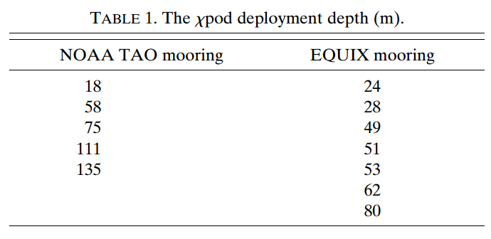
Read χpod data#
equix_iop = xr.load_dataset("/home/deepak/datasets/microstructure/osu/equix/iop.nc")
equix_iop.coords["kind"] = ("depth", ["APL"] * equix_iop.sizes["depth"])

tao_iop = (
    xr.load_dataset("/home/deepak/datasets/microstructure/osu/equix/tao_may08.nc")
    .reindex(time=equix_iop.time)
    .drop_sel(depth=[39, 84])
)
tao_iop.coords["kind"] = ("depth", ["TAO"] * tao_iop.sizes["depth"])

# depths are quite different so simple merge works.
# clusters of 3 χpods are also separated
iop_ = xr.merge([tao_iop, equix_iop])

iop = iop_[["theta", "chi", "eps", "dTdz"]].coarsen(time=10, boundary="trim").mean()
iop["salt"] = 35 * xr.ones_like(iop.theta)
iop["salt"].attrs = {"standard_name": "sea_water_salinity"}
iop["theta"].attrs = {"standard_name": "sea_water_temperature"}
iop["pres"] = iop.depth
iop["pres"].attrs = {"standard_name": "sea_water_pressure"}
iop.coords["latitude"] = 0
iop.coords["longitude"] = -140
iop = iop.cf.guess_coord_axis()
iop = ed.sections.add_ancillary_variables(iop)
iop
<xarray.Dataset>
Dimensions:             (depth: 12, time: 2256)
Coordinates:
  * depth               (depth) int64 18 24 28 49 51 53 59 62 69 80 124 150
  * time                (time) datetime64[ns] 2008-10-24T07:05:00 ... 2008-11...
    unit                (depth) float64 313.0 nan nan nan ... nan 327.0 321.0
    kind                (depth) object 'TAO' 'APL' 'APL' ... 'APL' 'TAO' 'TAO'
    actual_depth        (depth, time) float64 nan nan nan nan ... nan nan nan
    latitude            int64 0
    longitude           int64 -140
    reference_pressure  int64 0
Data variables: (12/15)
    theta               (depth, time) float64 24.49 24.51 24.5 ... 16.74 16.88
    chi                 (depth, time) float64 1.617e-06 3.078e-06 ... 2.275e-10
    eps                 (depth, time) float64 7.304e-06 1.578e-05 ... 1.673e-10
    Tz                  (depth, time) float64 0.002167 0.0036 ... 0.1626 0.01216
    salt                (depth, time) float64 35.0 35.0 35.0 ... 35.0 35.0 35.0
    pres                (depth) int64 18 24 28 49 51 53 59 62 69 80 124 150
    ...                  ...
    chi_masked          (depth, time) float64 1.617e-06 3.078e-06 ... 2.275e-10
    Krho                (depth, time) float64 0.02864 0.05469 ... 2.409e-07
    KrhoTz              (depth, time) float64 6.205e-05 0.0001969 ... 2.93e-09
    eps_chi             (depth, time) float64 4.392e-05 3.427e-05 ... 5.343e-10
    Kt                  (depth, time) float64 0.1722 0.1188 ... 7.692e-07
KtTz (depth, time) float64 0.0003731 0.0004276 ... 9.355e-09- depth: 12
- time: 2256
- depth(depth)int6418 24 28 49 51 ... 62 69 80 124 150
- axis :
- Z
- positive :
- down
array([ 18, 24, 28, 49, 51, 53, 59, 62, 69, 80, 124, 150])
- time(time)datetime64[ns]2008-10-24T07:05:00 ... 2008-11-...
- axis :
- T
- standard_name :
- time
array(['2008-10-24T07:05:00.000000000', '2008-10-24T07:15:00.000000000', '2008-10-24T07:25:00.000000000', ..., '2008-11-08T22:34:59.500000000', '2008-11-08T22:44:59.300000000', '2008-11-08T22:54:59.500000000'], dtype='datetime64[ns]') - unit(depth)float64313.0 nan nan ... nan 327.0 321.0
array([313., nan, nan, nan, nan, nan, 325., nan, 319., nan, 327., 321.]) - kind(depth)object'TAO' 'APL' 'APL' ... 'TAO' 'TAO'
array(['TAO', 'APL', 'APL', 'APL', 'APL', 'APL', 'TAO', 'APL', 'TAO', 'APL', 'TAO', 'TAO'], dtype=object) - actual_depth(depth, time)float64nan nan nan nan ... nan nan nan nan
array([[ nan, nan, nan, ..., nan, nan, nan], [ nan, nan, nan, ..., nan, nan, nan], [29.38945384, 29.40847237, 29.41894338, ..., nan, nan, nan], ..., [80.27413187, 80.30460324, 80.29368726, ..., 79.53041985, 79.39983229, 79.46079422], [ nan, nan, nan, ..., nan, nan, nan], [ nan, nan, nan, ..., nan, nan, nan]]) - latitude()int640
- units :
- degrees_north
- standard_name :
- latitude
array(0)
- longitude()int64-140
- units :
- degrees_east
- standard_name :
- longitude
array(-140)
- reference_pressure()int640
- units :
- dbar
array(0)
- theta(depth, time)float6424.49 24.51 24.5 ... 16.74 16.88
- standard_name :
- sea_water_temperature
- long_name :
- $θ$
array([[24.48868121, 24.51135426, 24.50407035, ..., 25.25005964, 25.26152833, 25.26864358], [ nan, nan, nan, ..., nan, nan, nan], [24.31340888, 24.31280316, 24.34244005, ..., nan, nan, nan], ..., [21.83992659, 22.01072639, 22.09691659, ..., 23.02981474, 22.97186977, 22.87988011], [17.24061852, 17.43636571, 17.37820315, ..., 18.41025824, 18.39259738, 18.39876725], [15.73683342, 15.73584339, 15.72846082, ..., 16.77826125, 16.74033692, 16.87978074]]) - chi(depth, time)float641.617e-06 3.078e-06 ... 2.275e-10
array([[1.61698769e-06, 3.07828509e-06, 1.21589035e-06, ..., 3.37009249e-07, 3.87328547e-08, 1.32696180e-07], [ nan, nan, nan, ..., nan, nan, nan], [7.38681268e-07, 4.89315946e-07, 6.05730390e-07, ..., nan, nan, nan], ..., [7.92941774e-10, 4.85757209e-10, 1.45324726e-10, ..., 1.90107136e-06, 7.69794928e-07, 5.20698876e-06], [1.18305903e-08, 1.14107335e-08, 8.84663921e-09, ..., 1.87420939e-08, 1.19233775e-08, 1.10975939e-07], [9.06700204e-10, 3.22719630e-10, 1.14630944e-10, ..., 1.44580309e-08, 1.35490665e-08, 2.27549757e-10]]) - eps(depth, time)float647.304e-06 1.578e-05 ... 1.673e-10
array([[7.30367896e-06, 1.57816952e-05, 3.25957771e-06, ..., 1.26132159e-07, 2.34226971e-08, 5.60676255e-08], [ nan, nan, nan, ..., nan, nan, nan], [3.78505241e-07, 1.63502359e-07, 2.69712581e-07, ..., nan, nan, nan], ..., [5.02126143e-11, 3.82326136e-11, 1.54215126e-11, ..., 9.96532729e-08, 5.50847009e-08, 2.92068902e-07], [1.19574166e-09, 4.91048750e-10, 3.99775333e-10, ..., 3.99957275e-09, 2.11157645e-09, 2.82719987e-08], [1.55235685e-09, 7.43387715e-10, 4.19472584e-10, ..., 3.41577787e-10, 4.84820790e-10, 1.67324893e-10]]) - Tz(depth, time)float640.002167 0.0036 ... 0.1626 0.01216
- long_name :
- $θ_z$
array([[0.00216671, 0.00359969, 0.00439116, ..., 0.01874413, 0.01139989, 0.01903666], [ nan, nan, nan, ..., nan, nan, nan], [0.02044969, 0.02488993, 0.01602949, ..., nan, nan, nan], ..., [0.09607571, 0.08039316, 0.07614283, ..., 0.12347199, 0.09730706, 0.10326908], [0.07234998, 0.19193251, 0.14527916, ..., 0.03063502, 0.03750828, 0.02220605], [0.00739581, 0.00298597, 0.00165814, ..., 0.10667042, 0.16258371, 0.01216215]]) - salt(depth, time)float6435.0 35.0 35.0 ... 35.0 35.0 35.0
- standard_name :
- sea_water_salinity
array([[35., 35., 35., ..., 35., 35., 35.], [35., 35., 35., ..., 35., 35., 35.], [35., 35., 35., ..., 35., 35., 35.], ..., [35., 35., 35., ..., 35., 35., 35.], [35., 35., 35., ..., 35., 35., 35.], [35., 35., 35., ..., 35., 35., 35.]]) - pres(depth)int6418 24 28 49 51 ... 62 69 80 124 150
- standard_name :
- sea_water_pressure
array([ 18, 24, 28, 49, 51, 53, 59, 62, 69, 80, 124, 150])
- pden(depth, time)float641.023e+03 1.023e+03 ... 1.026e+03
- standard_name :
- sea_water_potential_density
- units :
- kg/m3
- long_name :
- $ρ$
array([[1023.49682696, 1023.49002349, 1023.4922096 , ..., 1023.26616667, 1023.26265777, 1023.26048031], [ nan, nan, nan, ..., nan, nan, nan], [1023.54991871, 1023.55009956, 1023.54124758, ..., nan, nan, nan], ..., [1024.26695208, 1024.21924815, 1024.1950854 , ..., 1023.92971298, 1023.94639989, 1023.9728357 ], [1025.46173085, 1025.41467173, 1025.42868958, ..., 1025.17557125, 1025.17998035, 1025.17844032], [1025.81284475, 1025.81306855, 1025.81473714, ..., 1025.57254874, 1025.58146917, 1025.54860693]]) - gamma_n(time, depth)float6423.5 nan 23.56 ... 23.98 25.2 25.58
- standard_name :
- neutral_density
- units :
- kg/m3
- long_name :
- $γ_n$
array([[23.50218589, nan, 23.55547969, ..., 24.27662536, 25.48754086, 25.84732143], [23.49536447, nan, 23.55566107, ..., 24.2285371 , 25.43952853, 25.84755159], [23.49755633, nan, 23.54678334, ..., 24.20418316, 25.45382636, 25.84926762], ..., [23.27101104, nan, nan, ..., 23.9371228 , 25.19609975, 25.60091402], [23.26749511, nan, nan, ..., 23.95389985, 25.20058203, 25.6100379 ], [23.26531331, nan, nan, ..., 23.98048258, 25.19901642, 25.57643416]]) - N2(time, depth)float645.101e-05 5.101e-05 ... 0.0001389
- long_name :
- $N²$
array([[5.10060738e-05, 5.10060738e-05, 6.35895871e-05, ..., 2.02425487e-04, 1.81078298e-04, 1.32437048e-04], [5.77082564e-05, 5.77082564e-05, 6.79969423e-05, ..., 1.65691321e-04, 1.92246796e-04, 1.50195354e-04], [4.71138534e-05, 4.71138534e-05, 5.60296418e-05, ..., 1.40225113e-04, 1.92458365e-04, 1.45563930e-04], ..., [3.14844515e-06, 3.14844515e-06, 3.14844515e-06, ..., 1.40740926e-04, 1.95381185e-04, 1.49014181e-04], [2.71991202e-06, 2.71991202e-06, 2.71991202e-06, ..., 1.49465342e-04, 1.95461846e-04, 1.50722783e-04], [9.01642817e-07, 9.01642817e-07, 9.01642817e-07, ..., 1.37624045e-04, 1.85774695e-04, 1.38929384e-04]]) - chi_masked(depth, time)float641.617e-06 3.078e-06 ... 2.275e-10
array([[1.61698769e-06, 3.07828509e-06, 1.21589035e-06, ..., 3.37009249e-07, 3.87328547e-08, 1.32696180e-07], [ nan, nan, nan, ..., nan, nan, nan], [7.38681268e-07, 4.89315946e-07, 6.05730390e-07, ..., nan, nan, nan], ..., [7.92941774e-10, 4.85757209e-10, 1.45324726e-10, ..., 1.90107136e-06, 7.69794928e-07, 5.20698876e-06], [1.18305903e-08, 1.14107335e-08, 8.84663921e-09, ..., 1.87420939e-08, 1.19233775e-08, 1.10975939e-07], [9.06700204e-10, 3.22719630e-10, 1.14630944e-10, ..., 1.44580309e-08, 1.35490665e-08, 2.27549757e-10]]) - Krho(depth, time)float640.02864 0.05469 ... 2.409e-07
- long_name :
- $K_ρ$
- units :
- m²/s
array([[2.86384676e-02, 5.46947567e-02, 1.38370245e-02, ..., 8.01234599e-03, 1.72231284e-03, nan], [ nan, nan, nan, ..., nan, nan, nan], [1.19046296e-03, 4.80910916e-04, 9.62749616e-04, ..., nan, nan, nan], ..., [4.96109607e-08, 4.61492050e-08, 2.19953648e-08, ..., 1.41612359e-04, 7.37089955e-05, 4.24444583e-04], [1.32069019e-06, 5.10852467e-07, 4.15440850e-07, ..., 4.09412273e-06, 2.16060218e-06, 3.04368674e-05], [2.34429395e-06, 9.89894422e-07, 5.76341385e-07, ..., 4.58450041e-07, 6.43327810e-07, 2.40877614e-07]]) - KrhoTz(depth, time)float646.205e-05 0.0001969 ... 2.93e-09
- long_name :
- $K_ρ θ_z$
- units :
- m²/s
array([[6.20512416e-05, 1.96884208e-04, 6.07606243e-05, ..., 1.50184432e-04, 1.96341847e-05, nan], [ nan, nan, nan, ..., nan, nan, nan], [2.43446016e-05, 1.19698396e-05, 1.54323843e-05, ..., nan, nan, nan], ..., [4.76640835e-09, 3.71008054e-09, 1.67478940e-09, ..., 1.74851592e-05, 7.17240542e-06, 4.38319995e-05], [9.55519038e-08, 9.80491939e-08, 6.03548997e-08, ..., 1.25423548e-07, 8.10404746e-08, 6.75882559e-07], [1.73379602e-08, 2.95579280e-09, 9.55654969e-10, ..., 4.89030562e-08, 1.04594619e-07, 2.92958906e-09]]) - eps_chi(depth, time)float644.392e-05 3.427e-05 ... 5.343e-10
- long_name :
- $ε_χ$
- units :
- W/kg
array([[4.39204941e-05, 3.42733395e-05, 7.42718103e-06, ..., 7.55000980e-09, 2.02662179e-09, nan], [ nan, nan, nan, ..., nan, nan, nan], [2.80808037e-07, 1.34267644e-07, 3.30215814e-07, ..., nan, nan, nan], ..., [4.34729668e-11, 3.11329873e-11, 8.78713397e-12, ..., 4.38754886e-08, 3.03785387e-08, 1.67988825e-07], [1.02314230e-09, 1.48872889e-10, 2.01673320e-10, ..., 9.75448637e-09, 4.14139798e-09, 1.04523229e-07], [5.48834424e-09, 1.35910080e-08, 1.51723558e-08, ..., 4.73356982e-10, 1.93140901e-10, 5.34305893e-10]]) - Kt(depth, time)float640.1722 0.1188 ... 7.692e-07
- long_name :
- $K_T$
- units :
- m²/s
array([[1.72216722e-01, 1.18781407e-01, 3.15286503e-02, ..., 4.79602435e-04, 1.49021128e-04, 1.83082601e-04], [ nan, nan, nan, ..., nan, nan, nan], [8.83188741e-04, 3.94922594e-04, 1.17871828e-03, ..., nan, nan, nan], ..., [4.29520684e-08, 3.75795028e-08, 1.25328962e-08, ..., 6.23492963e-05, 4.06496093e-05, 2.44127144e-04], [1.13005514e-06, 1.54876848e-07, 2.09576050e-07, ..., 9.98508261e-06, 4.23755129e-06, 1.12526874e-04], [8.28823103e-06, 1.80977742e-05, 2.08463124e-05, ..., 6.35318034e-07, 2.56286272e-07, 7.69176219e-07]]) - KtTz(depth, time)float640.0003731 0.0004276 ... 9.355e-09
- long_name :
- $K_t θ_z$
- units :
- m²/s
array([[3.73143618e-04, 4.27576329e-04, 1.38447430e-04, ...,
        8.98972904e-06, 1.69882514e-06, 3.48528061e-06],
       [           nan,            nan,            nan, ...,
                   nan,            nan,            nan],
       [1.80609382e-05, 9.82959620e-06, 1.88942515e-05, ...,
                   nan,            nan,            nan],
       ...,
       [4.12665054e-09, 3.02113509e-09, 9.54290234e-10, ...,
        7.69839143e-06, 3.95549384e-06, 2.52107843e-05],
       [8.17594623e-08, 2.97259016e-08, 3.04470336e-08, ...,
        3.05893246e-07, 1.58943266e-07, 2.49877725e-06],
       [6.12982086e-08, 5.40393699e-08, 3.45661141e-08, ...,
        6.77696384e-08, 4.16679717e-08, 9.35483463e-09]])
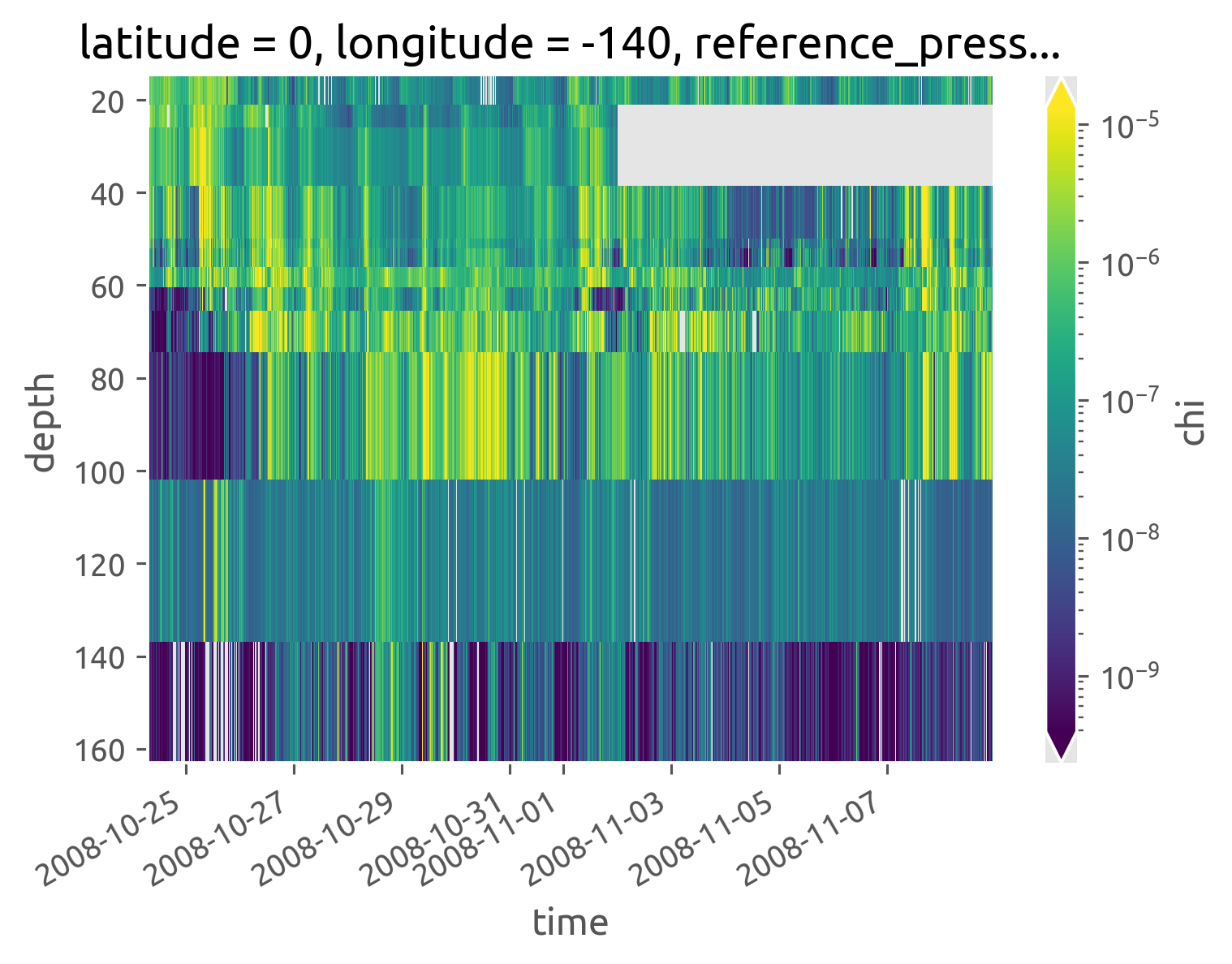
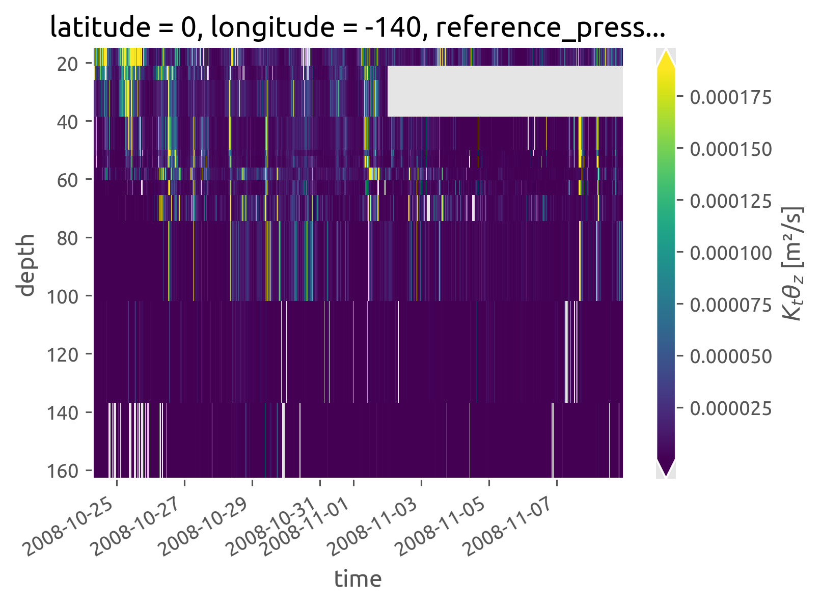
iop.chi.cf.plot(robust=True, norm=mpl.colors.LogNorm())
<matplotlib.collections.QuadMesh at 0x7fccfd0e8ee0>
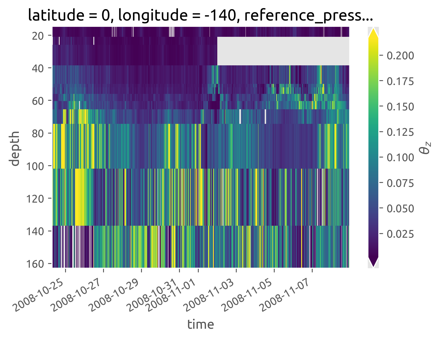
Do ancillary variables#
iop.Tz.cf.plot(robust=True)
<matplotlib.collections.QuadMesh at 0x7fccfcf57b20>
iop.KtTz.cf.plot(robust=True)
<matplotlib.collections.QuadMesh at 0x7fccfce35a00>
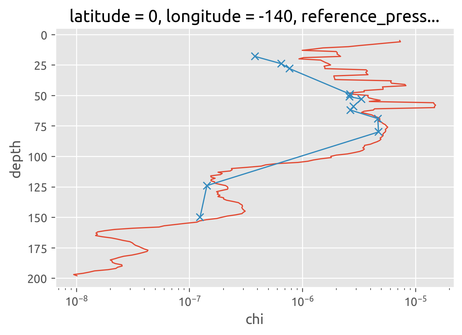
IOP: χpod vs Chameleon#
Not sure why this does not totally agree with Perlin & Moum
chameleon.chi.mean("time").rolling(depth=5, center=True).mean().cf.plot()
iop.chi.mean("time").cf.plot(marker="x", xscale="log")
[<matplotlib.lines.Line2D at 0x7fccfcd17ca0>]
bin-averaging in density space#
cham_dens = ed.sections.bin_average_vertical(chameleon, "neutral_density", bins)

iop_dens = ed.sections.bin_average_vertical(
    iop.where(iop.Tz > 5e-3), "neutral_density", bins, skip_fits=True
)
tao_dens = ed.sections.bin_average_vertical(
    iop.where(iop.Tz > 5e-3).query(depth="kind == 'TAO'"),
    "neutral_density",
    bins,
    skip_fits=True,
)

apl_dens = ed.sections.bin_average_vertical(
    iop.where(iop.Tz > 5e-3).query(depth="kind == 'APL'"),
    "neutral_density",
    bins,
    skip_fits=True,
)
chipod_dens = xr.concat([iop_dens, tao_dens, apl_dens], dim="kind")
chipod_dens["kind"] = ["iop", "TAO", "APL"]

# χpod depths are useless as a mean pressure
# we need to remap using the mean; here we use chameleon for now
# could use Argo et al later
chipod_dens = chipod_dens.rename({"pres": "χpod_pres"})
chipod_dens.coords["pres"] = cham_dens["pres"].reset_coords(drop=True)

for var in cham_dens:
    cham_dens[var].attrs["coordinates"] = "pres"
cham_dens.num_obs.cf.plot(y="pres")
chipod_dens.num_obs.sel(kind="iop").cf.plot(y="pres", xscale="log")
dcpy.plots.linex([cham_dens.num_obs.median() / 3, chipod_dens.num_obs.median() / 3])
final result#
This was wrong earlier :X. I forgot to do χ/2 with the χpod estimate
χpods say no difference i.e. there doesn’t seem to be any eddy stirring
Old notes: Mostly agree.
It looks like the biggest disagreement is between 100m and 120m ≈ EUCmax.
Note that I have used the chameleon \(∂_zθ^m\)
crosses need to be moved one half-bin width down
chipodmask = chipod_dens.num_obs > chipod_dens.num_obs.median() / 3
chammask = cham_dens.num_obs > cham_dens.num_obs.median() / 3

ed.sections.plot_var_prod_diss(cham_dens.where(chammask))
(chipod_dens.chi / 2).where(chipodmask).sel(kind="iop").cf.plot(
    y="pres", color="r", ls="none", marker="x"
)
(chipod_dens.where(chipodmask).KtTz * cham_dens.dTdz_m).sel(kind="iop").cf.plot(
    y="pres", marker="x", ls="none", color="k"
)
plt.title("EQUIX IOP")
hdl = dcpy.plots.liney(chameleon.eucmax.mean().values, label="$z_{EUC}$")
chipod_dens.where(chipod_dens.num_obs > 600).sel(kind="iop").chi.cf.plot.step(y="pres")
chipod_dens.where(chipod_dens.num_obs > 250).sel(kind="TAO").chi.cf.plot.step(y="pres")
chipod_dens.where(chipod_dens.num_obs > 250).sel(kind="APL").chi.cf.plot.step(y="pres")
EQUIX EOP#
[ ] need salinity
[ ] merge in TAO
[ ] need to preserve time dimension while grouping
equix_eop = xr.open_dataset(
    "/home/deepak/datasets/microstructure/osu/equix/hourly_eop.nc"
).rename({"dTdz": "Tz"})
equix_eop["depth"] = equix_eop.depth.data.astype(int)
equix_eop["salt"] = 35 * xr.ones_like(equix_eop.theta)
equix_eop["salt"].attrs = {"standard_name": "sea_water_salinity"}
equix_eop["T"] = dcpy.eos.temp(equix_eop.salt, equix_eop.theta, equix_eop.depth)
equix_eop.coords["pres"] = dcpy.eos.pres(equix_eop.depth, 0)
equix_eop.coords["latitude"] = 0
equix_eop.coords["longitude"] = -140
equix_eop = equix_eop.cf.guess_coord_axis()
equix_eop["gamma_n"] = dcpy.oceans.neutral_density(equix_eop)
equix_eop["pden"] = dcpy.eos.pden(equix_eop.salt, equix_eop.theta, 0)
equix_eop.attrs["name"] = "EQUIX"

tao = xr.open_dataset("/home/deepak/datasets/microstructure/osu/equix/hourly_tao.nc")
tao.attrs["name"] = "TAO"

tao_eop = dcpy.util.slice_like(tao, equix_eop.time).drop_sel(depth=[39, 84])
eop = xr.merge([tao_eop, equix_eop])
eop
<xarray.Dataset>
Dimensions:             (depth: 11, time: 2692)
Coordinates:
  * depth               (depth) int64 18 25 29 47 49 58 59 69 76 124 150
  * time                (time) datetime64[ns] 2008-11-11T05:00:00 ... 2009-03...
    unit                (depth) float64 313.0 315.0 328.0 ... 304.0 327.0 321.0
    pres                (depth) float64 nan 25.15 29.17 47.28 ... 76.47 nan nan
    latitude            int64 0
    longitude           int64 -140
    reference_pressure  int64 0
Data variables:
    theta               (time, depth) float64 24.77 24.62 24.51 ... 18.66 15.89
    chi                 (time, depth) float64 2.222e-07 7.709e-08 ... 2.5e-07
    eps                 (time, depth) float64 4.368e-07 6.169e-08 ... 7.051e-09
    Kt                  (time, depth) float64 0.008625 0.0002651 ... 3.797e-06
    Jq                  (time, depth) float64 98.86 13.11 40.81 ... 1.153 2.633
    dTdz                (time, depth) float64 0.008565 nan ... 0.06073 0.2235
    Tz                  (time, depth) float64 nan 0.01206 0.005363 ... nan nan
    KtTz                (time, depth) float64 nan 3.196e-06 ... nan nan
    salt                (time, depth) float64 nan 35.0 35.0 ... 35.0 nan nan
    T                   (time, depth) float64 nan 24.62 24.52 ... 21.78 nan nan
    gamma_n             (time, depth) float64 nan 23.46 23.49 ... 24.29 nan nan
pden (time, depth) float64 nan 1.023e+03 ... nan nan- depth: 11
- time: 2692
- depth(depth)int6418 25 29 47 49 58 59 69 76 124 150
- positive :
- down
array([ 18, 25, 29, 47, 49, 58, 59, 69, 76, 124, 150])
- time(time)datetime64[ns]2008-11-11T05:00:00 ... 2009-03-...
array(['2008-11-11T05:00:00.000000000', '2008-11-11T06:00:00.000000000', '2008-11-11T07:00:00.000000000', ..., '2009-03-03T06:00:00.000000000', '2009-03-03T07:00:00.000000000', '2009-03-03T08:00:00.000000000'], dtype='datetime64[ns]') - unit(depth)float64313.0 315.0 328.0 ... 327.0 321.0
array([313., 315., 328., 314., 204., 205., 325., 319., 304., 327., 321.])
- pres(depth)float64nan 25.15 29.17 ... 76.47 nan nan
- axis :
- Z
- standard_name :
- sea_water_pressure
- units :
- dbar
array([ nan, 25.15028761, 29.17459466, 47.28486766, 49.29721026, 58.35297481, nan, nan, 76.46559818, nan, nan]) - latitude()int640
- units :
- degrees_north
- standard_name :
- latitude
array(0)
- longitude()int64-140
- units :
- degrees_east
- standard_name :
- longitude
array(-140)
- reference_pressure()int640
- units :
- dbar
array(0)
- theta(time, depth)float6424.77 24.62 24.51 ... 18.66 15.89
array([[24.7671738 , 24.61707766, 24.51454595, ..., 20.76772423, 17.54687406, 16.35304952], [24.71691331, 24.65918957, 24.53396839, ..., 21.43123331, 17.30524057, 16.28518759], [24.68849958, 24.66569051, 24.54497897, ..., 21.3059526 , 16.89465195, 16.03821869], ..., [25.60260047, 25.18074719, 24.18486 , ..., 21.11633696, 18.12848966, 15.14817704], [25.58889999, 25.20439481, 24.30577217, ..., 21.11266278, 18.55093016, 16.00948797], [25.55872526, nan, nan, ..., 21.76088171, 18.65550553, 15.89052162]]) - chi(time, depth)float642.222e-07 7.709e-08 ... 2.5e-07
array([[2.22196874e-07, 7.70923322e-08, 1.06762781e-07, ..., 2.07682746e-06, 3.25108273e-08, 1.55838828e-10], [2.90461897e-07, 1.96698890e-07, 2.96826853e-07, ..., 6.53712800e-07, 1.90470335e-08, 1.28388162e-09], [3.45599604e-07, 1.30622032e-07, 2.53211147e-07, ..., 1.08080336e-07, 3.29074287e-08, 9.83816236e-10], ..., [9.79353037e-08, 2.94532554e-08, 4.36463857e-08, ..., 3.06965859e-09, 2.93626713e-08, 2.44092247e-09], [3.96324085e-07, 7.83073901e-08, 4.68988801e-08, ..., 5.29027402e-08, 2.09588492e-08, 1.01333535e-08], [3.27658825e-07, 1.17872698e-07, 1.60111262e-07, ..., 2.59367495e-10, 2.65507442e-08, 2.49968249e-07]]) - eps(time, depth)float644.368e-07 6.169e-08 ... 7.051e-09
array([[4.36819496e-07, 6.16871908e-08, 2.34990808e-07, ..., 5.60776529e-08, 6.63909399e-09, 1.46473911e-10], [5.24716616e-07, 1.04931162e-07, 2.64477547e-07, ..., 3.75679530e-08, 1.56004829e-09, 3.62426473e-10], [6.52470515e-07, 9.29881821e-08, 3.41733374e-07, ..., 8.22501662e-09, 3.06125773e-08, 7.45567639e-11], ..., [8.28483182e-08, 1.08852079e-08, 5.79175229e-09, ..., 1.69291656e-10, 1.75947123e-09, 1.16256972e-10], [3.29818570e-07, 1.42536890e-08, 8.83651226e-09, ..., 2.49331360e-09, 2.30391210e-09, 2.97153055e-10], [3.00827923e-07, nan, nan, ..., 1.87530821e-11, 3.46467353e-09, 7.05050379e-09]]) - Kt(time, depth)float640.008625 0.0002651 ... 3.797e-06
array([[8.62471755e-03, 2.65050762e-04, 1.85625941e-03, ..., 2.35650893e-05, 2.38957158e-05, 2.69293784e-06], [8.15907606e-03, 4.18117793e-04, 1.74008330e-03, ..., 2.70805314e-05, 2.52299719e-06, 1.04893334e-05], [1.18472130e-02, 3.11640697e-04, 1.47039376e-03, ..., 6.07437177e-06, 5.67100026e-04, 9.43926757e-08], ..., [1.14225162e-03, 3.35356161e-05, 7.44277103e-06, ..., 1.36671789e-07, 1.58624476e-06, 2.79842509e-07], [2.65002522e-03, 1.35610061e-04, 1.36038013e-05, ..., 2.29850076e-06, 4.69722032e-06, 3.28592874e-07], [2.51514524e-03, nan, nan, ..., 1.17059832e-08, 6.77179084e-06, 3.79661382e-06]]) - Jq(time, depth)float6498.86 13.11 40.81 ... 1.153 2.633
array([[9.88587966e+01, 1.31050590e+01, 4.08129636e+01, ..., 2.02816654e+01, 2.05496959e+00, 5.00475267e-02], [1.21099902e+02, 2.62917285e+01, 6.58878707e+01, ..., 1.21980650e+01, 5.42246355e-01, 1.30378418e-01], [1.58355161e+02, 1.84971220e+01, 5.59405968e+01, ..., 2.34905338e+00, 7.83586837e+00, 2.73749275e-02], ..., [2.02039838e+01, 2.88130117e+00, 1.65238153e+00, ..., 5.93817971e-02, 5.95468303e-01, 4.50060052e-02], [8.21618293e+01, 9.44748454e+00, 2.31568901e+00, ..., 1.01095138e+00, 7.55538777e-01, 1.09298345e-01], [6.14414009e+01, nan, nan, ..., 5.05161891e-03, 1.15349378e+00, 2.63263460e+00]]) - dTdz(time, depth)float640.008565 nan nan ... 0.06073 0.2235
array([[0.00856479, nan, nan, ..., nan, 0.05193922, 0.01156739], [0.00665374, nan, nan, ..., nan, 0.10475808, 0.03862674], [0.00519374, nan, nan, ..., nan, 0.06882454, 0.0740183 ], ..., [0.01834773, nan, nan, ..., nan, 0.11504129, 0.08116051], [0.01239896, nan, nan, ..., nan, 0.10398424, 0.15868845], [0.01317509, nan, nan, ..., nan, 0.0607282 , 0.22350066]]) - Tz(time, depth)float64nan 0.01206 0.005363 ... nan nan
array([[ nan, 0.01205941, 0.0053626 , ..., 0.20991848, nan, nan], [ nan, 0.01533687, 0.00923531, ..., 0.10986261, nan, nan], [ nan, 0.01447659, 0.00927918, ..., 0.09432084, nan, nan], ..., [ nan, 0.02095552, 0.05414917, ..., 0.10597187, nan, nan], [ nan, 0.01699184, 0.04151797, ..., 0.1072758 , nan, nan], [ nan, nan, nan, ..., 0.10525405, nan, nan]]) - KtTz(time, depth)float64nan 3.196e-06 9.954e-06 ... nan nan
- long_name :
- $χ$
- units :
- °C²/s
array([[ nan, 3.19635585e-06, 9.95438137e-06, ..., 4.94674765e-06, nan, nan], [ nan, 6.41261670e-06, 1.60702124e-05, ..., 2.97513781e-06, nan, nan], [ nan, 4.51149316e-06, 1.36440480e-05, ..., 5.72939848e-07, nan, nan], ..., [ nan, 7.02756383e-07, 4.03019885e-07, ..., 1.44833651e-08, nan, nan], [ nan, 2.30426452e-06, 5.64802199e-07, ..., 2.46573507e-07, nan, nan], [ nan, nan, nan, ..., 1.23210217e-09, nan, nan]]) - salt(time, depth)float64nan 35.0 35.0 35.0 ... 35.0 nan nan
- standard_name :
- sea_water_salinity
array([[nan, 35., 35., ..., 35., nan, nan], [nan, 35., 35., ..., 35., nan, nan], [nan, 35., 35., ..., 35., nan, nan], ..., [nan, 35., 35., ..., 35., nan, nan], [nan, 35., 35., ..., 35., nan, nan], [nan, 35., 35., ..., 35., nan, nan]]) - T(time, depth)float64nan 24.62 24.52 ... 21.78 nan nan
- standard_name :
- sea_water_temperature
- units :
- degC
- description :
- ITS-90
array([[ nan, 24.6224332 , 24.52073992, ..., 20.78213751, nan, nan], [ nan, 24.66455181, 24.54016595, ..., 21.44597498, nan, nan], [ nan, 24.67105378, 24.55117856, ..., 21.32063239, nan, nan], ..., [ nan, 25.1861922 , 24.19099307, ..., 21.130923 , nan, nan], [ nan, 25.20984357, 24.31192759, ..., 21.127247 , nan, nan], [ nan, nan, nan, ..., 21.77578588, nan, nan]]) - gamma_n(time, depth)float64nan 23.46 23.49 ... 24.29 nan nan
- standard_name :
- neutral_density
- units :
- kg/m3
- long_name :
- $γ_n$
array([[ nan, 23.46239095, 23.49331767, ..., 24.56912943, nan, nan], [ nan, 23.44967624, 23.48746939, ..., 24.38645079, nan, nan], [ nan, 23.44771222, 23.48415276, ..., 24.42120791, nan, nan], ..., [ nan, 23.29108124, 23.59216142, ..., 24.47357929, nan, nan], [ nan, 23.28384131, 23.55600433, ..., 24.47459131, nan, nan], [ nan, nan, nan, ..., 24.29440553, nan, nan]]) - pden(time, depth)float64nan 1.023e+03 1.023e+03 ... nan nan
- standard_name :
- sea_water_potential_density
- units :
- kg/m3
array([[          nan, 1023.45708559, 1023.48791156, ..., 1024.55686465,
                  nan,           nan],
       [          nan, 1023.4444009 , 1023.48207856, ..., 1024.37586006,
                  nan,           nan],
       [          nan, 1023.44244149, 1023.47877051, ..., 1024.41031435,
                  nan,           nan],
       ...,
       [          nan, 1023.2861544 , 1023.5864724 , ..., 1024.46221624,
                  nan,           nan],
       [          nan, 1023.27892932, 1023.55042437, ..., 1024.46321902,
                  nan,           nan],
       [          nan,           nan,           nan, ..., 1024.28458651,
                  nan,           nan]])
eccoT_full, edges = ed.estimate_gradients(ecco, bins, bin_var="gamma_n", debug=True)
eccoT = eccoT_full.interp(lat=0)
argoT_full, _ = ed.estimate_gradients(argo, bins, bin_var="gamma_n", debug=True)
argoT = argoT_full.interp(lat=0)
eccoT
<xarray.Dataset>
Dimensions:         (bounds: 2, gamma_n: 11)
Coordinates:
    lon             float64 220.2
  * gamma_n         (gamma_n) float64 23.54 23.67 23.84 ... 25.96 26.16 26.28
    gamma_n_bounds  (bounds, gamma_n) float64 23.49 23.59 23.74 ... 26.23 26.33
    dz_remapped     (gamma_n) float64 7.004 8.579 10.3 13.2 ... 21.8 18.04 17.01
    pres            (gamma_n) float64 57.03 64.82 74.26 ... 174.0 193.9 211.4
    y               float64 0.0
    lat             int64 0
Dimensions without coordinates: bounds
Data variables:
    Tmean           (gamma_n) float64 24.9 24.59 24.12 ... 15.3 14.32 13.66
    dTdy            (gamma_n) float64 -3.753e-06 -3.315e-06 ... -1.896e-06
dTdz (gamma_n) float64 0.03738 0.04391 ... 0.04075 0.03307- bounds: 2
- gamma_n: 11
- lon()float64220.2
- units :
- degrees_east
- standard_name :
- longitude
array(220.25)
- gamma_n(gamma_n)float6423.54 23.67 23.84 ... 26.16 26.28
- bounds :
- gamma_n_bounds
- standard_name :
- neutral_density
- units :
- kg/m3
- long_name :
- $γ_n$
array([23.540451, 23.665252, 23.835972, 24.078303, 24.427783, 24.864182, 25.285968, 25.658478, 25.963018, 26.156028, 26.276818]) - gamma_n_bounds(bounds, gamma_n)float6423.49 23.59 23.74 ... 26.23 26.33
array([[23.487837 , 23.59306484, 23.73743935, 23.93450429, 24.22210138, 24.63346371, 25.09490123, 25.47703517, 25.83992123, 26.08611433, 26.22594153], [23.59306484, 23.73743935, 23.93450429, 24.22210138, 24.63346371, 25.09490123, 25.47703517, 25.83992123, 26.08611433, 26.22594153, 26.32769379]]) - dz_remapped(gamma_n)float647.004 8.579 10.3 ... 18.04 17.01
array([ 7.00436683, 8.57938591, 10.2962578 , 13.20114123, 16.24706725, 17.14768799, 16.14896516, 20.91204945, 21.80453402, 18.04137588, 17.01059992]) - pres(gamma_n)float6457.03 64.82 74.26 ... 193.9 211.4
- axis :
- Z
- long_name :
- Pressure at bin centers
array([ 57.02558807, 64.81746445, 74.2552863 , 86.00398582, 100.72809006, 117.42546768, 134.07379426, 152.60430157, 173.96259331, 193.88554826, 211.41153616]) - y()float640.0
- units :
- degrees_north
- standard_name :
- latitude
- axis :
- Y
array(0.)
- lat()int640
- units :
- degrees_north
- standard_name :
- latitude
array(0)
- Tmean(gamma_n)float6424.9 24.59 24.12 ... 14.32 13.66
array([24.89646852, 24.58522831, 24.12117364, 23.35246227, 22.06281062, 20.28590038, 18.45363735, 16.75850973, 15.30144443, 14.31697906, 13.65788513]) - dTdy(gamma_n)float64-3.753e-06 ... -1.896e-06
array([-3.75252259e-06, -3.31527389e-06, -4.29448794e-06, -3.92886946e-06, -4.19549862e-06, -4.14071104e-06, -3.51199979e-06, -3.04193781e-06, -2.67605539e-06, -2.23184697e-06, -1.89600616e-06]) - dTdz(gamma_n)float640.03738 0.04391 ... 0.04075 0.03307
array([0.03737798, 0.04390691, 0.05574944, 0.07373562, 0.09848518,
       0.11340485, 0.10533663, 0.08134383, 0.05599961, 0.04075305,
       0.03307156])
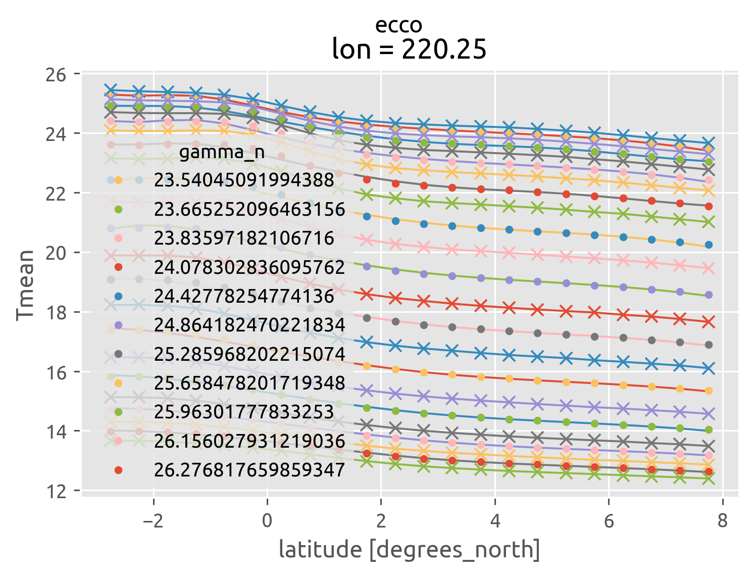
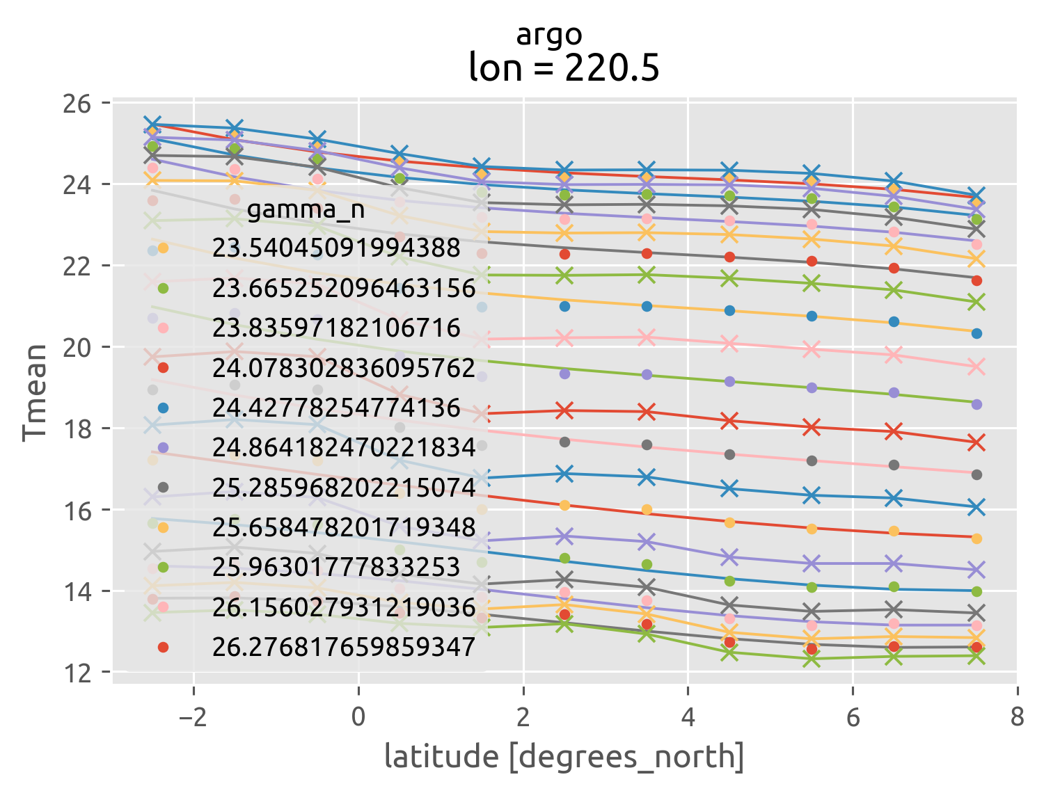
chipod_dens_df = ed.eddydiff.bin_avg_in_density_time(
    eop.where(eop.Tz > 5e-3), bins={"neutral_density": bins}, strftime="%Y"
)
chipod_dens = ed.sections.bin_average_vertical(
    eop.where(eop.Tz > 1e-2), "neutral_density", bins, skip_fits=True
)
chipod_dens
<xarray.Dataset>
Dimensions:             (bounds: 2, gamma_n: 11)
Coordinates:
  * gamma_n             (gamma_n) float64 23.54 23.66 23.84 ... 26.16 26.28
    pres                (gamma_n) float64 40.65 42.21 43.99 47.9 ... nan nan nan
    latitude            int64 0
    longitude           int64 -140
    reference_pressure  int64 0
    num_obs             (gamma_n) float64 1.412e+03 2.154e+03 3e+03 ... nan nan
    gamma_n_bounds      (bounds, gamma_n) float64 23.49 23.59 ... 26.23 26.33
Dimensions without coordinates: bounds
Data variables:
    theta               (gamma_n) float64 24.34 23.95 23.39 ... nan nan nan
    chi                 (gamma_n) float64 1.007e-06 1.207e-06 ... nan nan
    eps                 (gamma_n) float64 5.64e-07 6.304e-07 ... nan nan
    Kt                  (gamma_n) float64 0.0006162 0.0005668 ... nan nan
    Jq                  (gamma_n) float64 64.93 65.87 85.84 ... nan nan nan
    dTdz                (gamma_n) float64 nan nan nan nan ... nan nan nan nan
    Tz                  (gamma_n) float64 0.02894 0.03726 0.04573 ... nan nan
    KtTz                (gamma_n) float64 1.584e-05 1.607e-05 ... nan nan
    salt                (gamma_n) float64 35.0 35.0 35.0 35.0 ... nan nan nan
    T                   (gamma_n) float64 24.34 23.96 23.4 22.55 ... nan nan nan
    pden                (gamma_n) float64 1.024e+03 1.024e+03 ... nan nan
unit (gamma_n) float64 263.4 268.7 280.9 ... nan nan nan- bounds: 2
- gamma_n: 11
- gamma_n(gamma_n)float6423.54 23.66 23.84 ... 26.16 26.28
- bounds :
- gamma_n_bounds
- standard_name :
- neutral_density
- units :
- kg/m3
- long_name :
- $γ_n$
- positive :
- down
- axis :
- Z
array([23.5405, 23.665 , 23.836 , 24.0785, 24.4275, 24.864 , 25.286 , 25.6585, 25.963 , 26.156 , 26.277 ]) - pres(gamma_n)float6440.65 42.21 43.99 ... nan nan nan
- axis :
- Z
- standard_name :
- sea_water_pressure
- units :
- dbar
- positive :
- down
array([40.6532882 , 42.20682344, 43.99081006, 47.89577763, 58.78918219, 71.85424529, 76.3411128 , 76.46559818, nan, nan, nan]) - latitude()int640
- units :
- degrees_north
- standard_name :
- latitude
array(0)
- longitude()int64-140
- units :
- degrees_east
- standard_name :
- longitude
array(-140)
- reference_pressure()int640
- units :
- dbar
array(0)
- num_obs(gamma_n)float641.412e+03 2.154e+03 ... nan nan
- long_name :
- count(χ) in bins
array([1412., 2154., 3000., 3201., 2706., 1227., 291., 44., nan, nan, nan]) - gamma_n_bounds(bounds, gamma_n)float6423.49 23.59 23.74 ... 26.23 26.33
array([[23.488, 23.593, 23.737, 23.935, 24.222, 24.633, 25.095, 25.477,
        25.84 , 26.086, 26.226],
       [23.593, 23.737, 23.935, 24.222, 24.633, 25.095, 25.477, 25.84 ,
        26.086, 26.226, 26.328]])
- theta(gamma_n)float6424.34 23.95 23.39 ... nan nan nan
array([24.33620568, 23.95373623, 23.38739797, 22.54025035, 21.36912997, 19.84064311, 18.1079246 , 16.94043853, nan, nan, nan]) - chi(gamma_n)float641.007e-06 1.207e-06 ... nan nan
- long_name :
- $⟨χ⟩$
array([1.00676035e-06, 1.20739320e-06, 2.09414469e-06, 2.23668306e-06, 2.41148731e-06, 2.56997120e-06, 1.29140345e-06, 1.42195876e-07, nan, nan, nan]) - eps(gamma_n)float645.64e-07 6.304e-07 ... nan nan
- long_name :
- $⟨ε⟩$
array([5.64046118e-07, 6.30448618e-07, 8.55933719e-07, 7.21278682e-07, 5.16741915e-07, 1.03058597e-06, 4.14127154e-08, 1.20298045e-08, nan, nan, nan]) - Kt(gamma_n)float640.0006162 0.0005668 ... nan nan
array([6.16155953e-04, 5.66843408e-04, 5.84178231e-04, 3.82885879e-04, 1.55861249e-04, 8.95067006e-05, 3.32655416e-05, 9.01051173e-06, nan, nan, nan]) - Jq(gamma_n)float6464.93 65.87 85.84 ... nan nan nan
array([64.93288332, 65.86853422, 85.83694398, 72.69476679, 48.49071088, 40.3020619 , 14.25661326, 2.68465212, nan, nan, nan]) - dTdz(gamma_n)float64nan nan nan nan ... nan nan nan nan
array([nan, nan, nan, nan, nan, nan, nan, nan, nan, nan, nan])
- Tz(gamma_n)float640.02894 0.03726 0.04573 ... nan nan
array([0.028935 , 0.03725561, 0.04573312, 0.06634366, 0.09577629, 0.12496492, 0.16835783, 0.09970723, nan, nan, nan]) - KtTz(gamma_n)float641.584e-05 1.607e-05 ... nan nan
- long_name :
- $χ$
- units :
- °C²/s
array([1.58372886e-05, 1.60654962e-05, 2.09358400e-05, 1.77304309e-05, 1.18270027e-05, 9.82977120e-06, 3.47722275e-06, 6.54793200e-07, nan, nan, nan]) - salt(gamma_n)float6435.0 35.0 35.0 35.0 ... nan nan nan
- standard_name :
- sea_water_salinity
array([35., 35., 35., 35., 35., 35., 35., 35., nan, nan, nan])
- T(gamma_n)float6424.34 23.96 23.4 ... nan nan nan
- standard_name :
- sea_water_temperature
- units :
- degC
- description :
- ITS-90
array([24.3447923 , 23.96254794, 23.39642507, 22.54981791, 21.38042255, 19.85374412, 18.12098047, 16.95291962, nan, nan, nan]) - pden(gamma_n)float641.024e+03 1.024e+03 ... nan nan
- standard_name :
- sea_water_potential_density
- units :
- kg/m3
array([1023.54129546, 1023.65497933, 1023.8211931 , 1024.06493893, 1024.39215758, 1024.80268983, 1025.24461914, 1025.52821145, nan, nan, nan]) - unit(gamma_n)float64263.4 268.7 280.9 ... nan nan nan
array([263.35694051, 268.70009285, 280.855     , 274.47172759,
       265.44308943, 287.14425428, 303.31958763, 304.        ,
                nan,          nan,          nan])
eccoT["gamma_n"] = argoT["gamma_n"] = chipod_dens.gamma_n
(chipod_dens.chi / 2).cf.plot(y="gamma_n")
(chipod_dens.KtTz * eccoT.dTdz).cf.plot(y="gamma_n")
[<matplotlib.lines.Line2D at 0x7f05e3244820>]
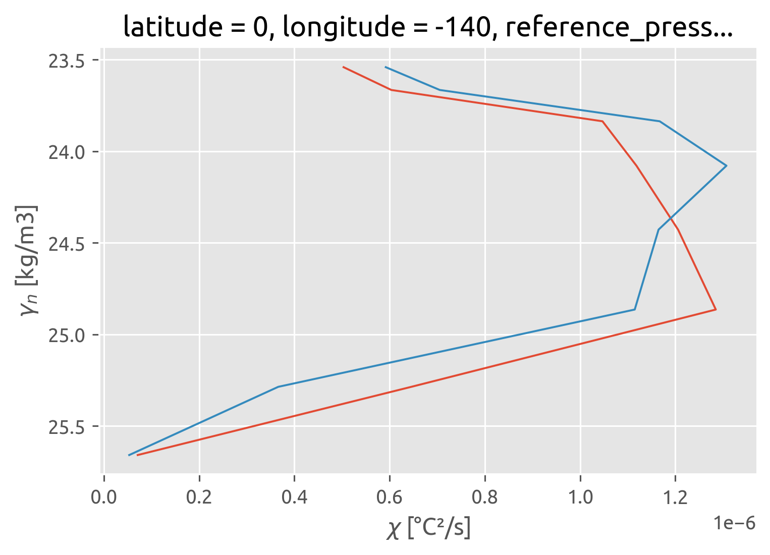
cole = cole.interp(lat=0, lon=220).set_coords("density_mean_depth")
cole_diff = xr.DataArray(
    np.interp(eccoT.gamma_n, cole.density_mean_depth, cole.diffusivity),
    dims="gamma_n",
    coords={"gamma_n": eccoT.gamma_n},
)

colegrad_pt = colegrad.interp(lat=0, lon=220)
cole_gradT = xr.DataArray(
    np.interp(eccoT.gamma_n, colegrad_pt.gamma_n, colegrad_pt.dTiso),
    dims="gamma_n",
    coords={"gamma_n": eccoT.gamma_n},
)
This plot shows local variance dissipation \(⟨χ⟩/2\) (chipod), local variance production \(⟨K_Tθ_z⟩⟨θ⟩\_z\) (chipod+climatology), and estimate of variance produced by eddy stirring using the Cole et al (2015) argo estimate \(K_e |⟨θ⟩\_y|²\) (cole + climatology).
The story seems to be consistent in that eddy stirring variance production is small.
Here I have used \(⟨θ⟩\_y\) at the equator from 1D spline fits to the mean field along isopycnals. Technically we would want a gradient between 1S and 5N (approx.). BUT it looks like the gradient is larger at the equator generally, so this might be an overestimate even.
I could redo the Cole estimate using argo points between 1°S and 5°N and combine with appropriate gradient (using their methodology) to get a better value possibly.
(chipod_dens.chi / 2).cf.plot(
    y="gamma_n", label="$⟨χ⟩/2$", color="r", size=4.5, aspect=1 / 1.4
)
# (chipod_dens.KtTz * cham_dens.dTdz_m).cf.plot(
#    y="gamma_n", xscale="log", label="$⟨K_T θ_z⟩ ⟨θ⟩_z^{cham}$"
# )
(chipod_dens.KtTz * eccoT.dTdz).cf.plot(
    y="gamma_n", xscale="log", color="k", ls="-", label="$⟨K_T θ_z⟩ ⟨θ⟩_z^{ecco}$"
)
(chipod_dens.KtTz * argoT.dTdz).cf.plot(
    y="gamma_n", xscale="log", color="k", ls="--", label="$⟨K_T θ_z⟩ ⟨θ⟩_z^{argo}$"
)
(cole_diff * cole_gradT**2).plot(
    y="gamma_n",
    color="k",
    ls="dashed",
    _labels=False,
    label="$Κ_e^{argo} |⟨θ⟩_y|²_{cole}$",
    ylim=(25.75, 23),
    xlim=(1e-10, None),
)
(cole_diff * argoT.dTdy**2).plot(
    y="gamma_n",
    color="k",
    ls=":",
    _labels=False,
    label="$Κ_e^{argo} |⟨θ⟩_y|²_{argo}$",
    ylim=(25.75, 23),
    xlim=(1e-10, None),
)
(cole_diff * eccoT.dTdy**2).plot(
    y="gamma_n",
    color="k",
    ls="-.",
    _labels=False,
    label="$Κ_e^{argo} |⟨θ⟩_y|²_{ecco}$",
    ylim=(25.75, 23),
    xlim=(1e-9, None),
)
plt.xticks([1e-9, 1e-8, 1e-7, 1e-6])
plt.legend(loc="upper left")
plt.title("")
plt.xlabel("Variance production/dissipation [°C²/s]")
Text(0.5, 0, 'Variance production/dissipation [°C²/s]')
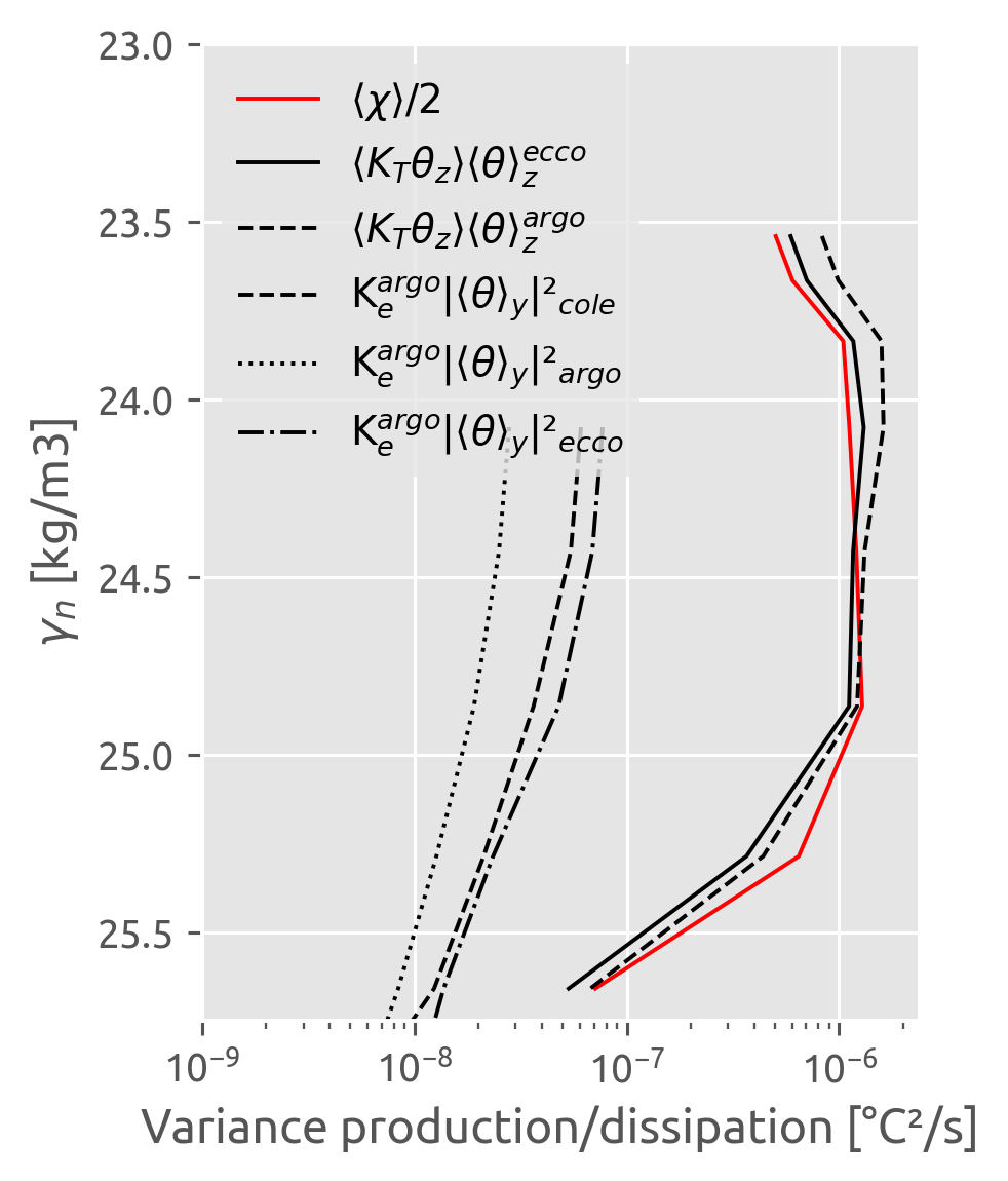
Uncertainties in estimating \(Κ_e^{argo} |⟨θ⟩\_y|²\)#
Using the spline gradient at 0 seems like a large value. I think we would want to estimate gradient between 1S and 5N. So the variance production estimate looks like an overestimate
xr.concat(
    [eccoT_full.dTdy, argoT_full.dTdy.interp(lat=eccoT_full.lat)], dim="kind"
).assign_coords(kind=["ecco", "argo"]).plot(col="kind", yincrease=False)
<xarray.plot.facetgrid.FacetGrid at 0x7fa55875d910>
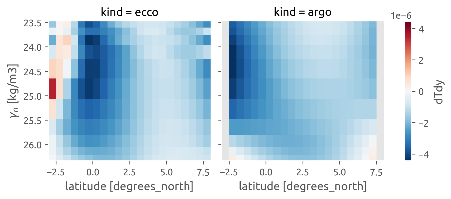
n-var groupby#
garr = np.array(tuple(tuple_groups))
out = np.arange(17 * 5, dtype=float).reshape((17, 5))
result = np.arange(55, dtype=float)
result[mask] = np.nan
out[(garr[:, 0], garr[:, 1])] = result
out
v1 = eop.gamma_n
v2 = eop.time.dt.month

to_group = ((v1, bins), v2)

factorized = []
groups = []
for var in to_group:
    if isinstance(var, tuple):
        # groupby_bins
        var, bins = var
        partitioned = pd.cut(var.data.ravel(), bins)
        cat = partitioned.codes
        uniques = partitioned.categories.values
    else:
        assert isinstance(var, xr.DataArray)  # really duck array
        cat, uniques = pd.factorize(var.data.ravel())

    groups.append(uniques)
    factorized.append(var.copy(data=cat.reshape(var.shape)))

factorized = xr.broadcast(*factorized)

ngroups = len(to_group)
iters = tuple(map(lambda x: x.flat, tuple(g.data for g in factorized)))
tuples = tuple(zip(*iters))
group_idx, tuple_groups = pd.factorize(tuples)
group_idx = group_idx.reshape(factorized[0].shape)
actual_groups = [tuple(g[i] for g, i in zip(groups, idx)) for idx in tuple_groups]
group_idx
from dask_groupby.core import chunk_reduce
result = chunk_reduce(eop.chi.data, group_idx, func=("mean",))
# result["groups"] = np.array(actual_groups)#[mask]
# result["mean"] = result["mean"]#[mask]

mask = [-1 not in tup for tup in tuple_groups.flat]
midx = pd.MultiIndex.from_tuples(actual_groups, names=["gamma_n_bins", "month"])[mask]
mean_chi = xr.DataArray(
    result["mean"][mask], dims="dim", coords={"dim": midx}
).unstack()
mean_chi
Comparing various \(T_z\) estimates#
First calculate dT/dz using chameleon after remappping to isopycnal bins.
Find mean T, mean z on the isopycnal surfaces. Then do dT/dz.
import xgcm

chamgrid = xgcm.Grid(chameleon, periodic=False, coords={"Z": {"center": "depth"}})
isoT = chamgrid.transform(
    chameleon.theta,
    axis="Z",
    target_data=chameleon.gamma_n,
    target=bins,
    method="linear",
)
zT = chamgrid.transform(
    chameleon.depth.broadcast_like(chameleon.gamma_n),
    axis="Z",
    target_data=chameleon.gamma_n,
    target=bins,
    method="linear",
)

cham_dens["dTdz_m_iso"] = (
    "gamma_n",
    (-1 * isoT.mean("time").diff("gamma_n") / zT.mean("time").diff("gamma_n")).data,
)
cham_dens.dTdz_m_iso.cf.plot(y="pres")
/home/deepak/miniconda3/envs/dcpy/lib/python3.8/site-packages/numba/np/ufunc/gufunc.py:151: RuntimeWarning: invalid value encountered in _interp_1d_linear
  return self.ufunc(*args, **kwargs)
[<matplotlib.lines.Line2D at 0x7f0c08438f70>]
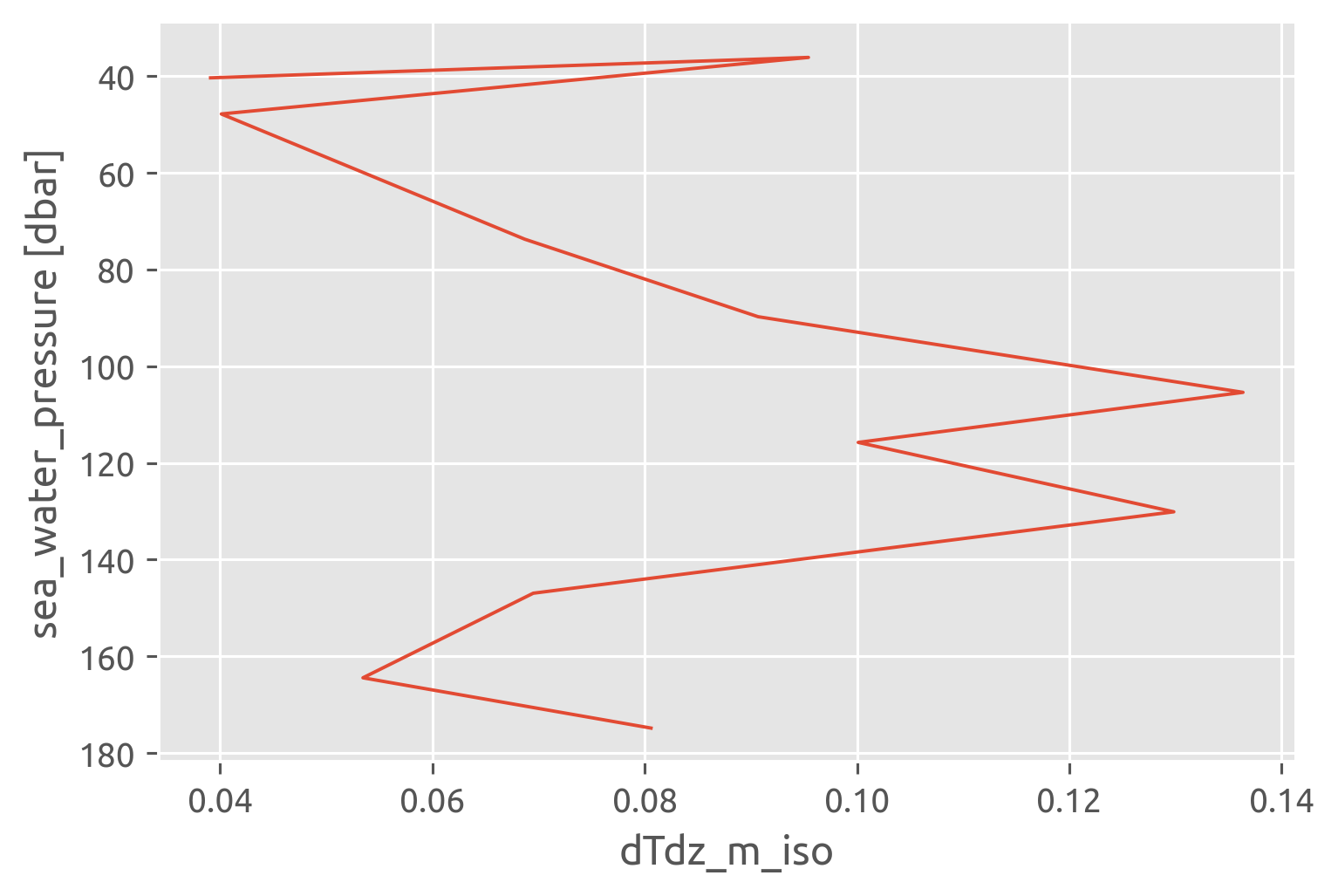
This figure compares estimates of the gradient in depth space and isopycnal space, from chameleon and various mean fields. Summary is that the fitting procedure of Polzin & Ferrari looks like an underestimate of the mean gradient. All other estimates are basically the same. That said, even though the fitting results in a lower value it’s not that low compared to all the other estimates.
Most interestingly the chameleon 2 week estimate is basically the same as the argo, ecco climatology estimates. This means that we can’t partition the variance dissipated :/
f, ax = plt.subplots(1, 2, sharex=True, constrained_layout=True)

y = "gamma_n"
plt.sca(ax[0])
(cham_dens.Tz).plot(y=y, label="cham mean Tz")
(cham_dens.dTdz_m).plot(y=y, label="cham fit Tz")
cham_dens.dTdz_m_iso.cf.plot(y=y, label="cham iso Tz")
eccoT.dTdz.plot.step(y=y, label="ecco iso Tz")
argoT.dTdz.plot.step(y=y, label="argo iso Tz")
ax[0].legend()

y = "pres"
plt.sca(ax[1])

chameleon.theta.mean("time").cf.differentiate("Z", follow_positive=True).cf.plot(
    label="cham diff"
)
ecco.Tmean.interp(lat=0).cf.differentiate("Z", follow_positive=True).cf.plot(
    label="ecco diff"
)
argo.Tmean.interp(lat=0).cf.differentiate("Z", follow_positive=True).cf.plot(
    label="argo diff"
)
(cham_dens.Tz).plot(y=y, label="cham mean Tz")
(cham_dens.dTdz_m).plot(y=y, label="cham fit Tz")
cham_dens.dTdz_m_iso.cf.plot(y=y, label="cham iso Tz")
eccoT.dTdz.plot.step(y=y, label="ecco iso Tz")
argoT.dTdz.plot.step(y=y, label="argo iso Tz")
ax[1].legend()
<matplotlib.legend.Legend at 0x7f0bb30fd370>
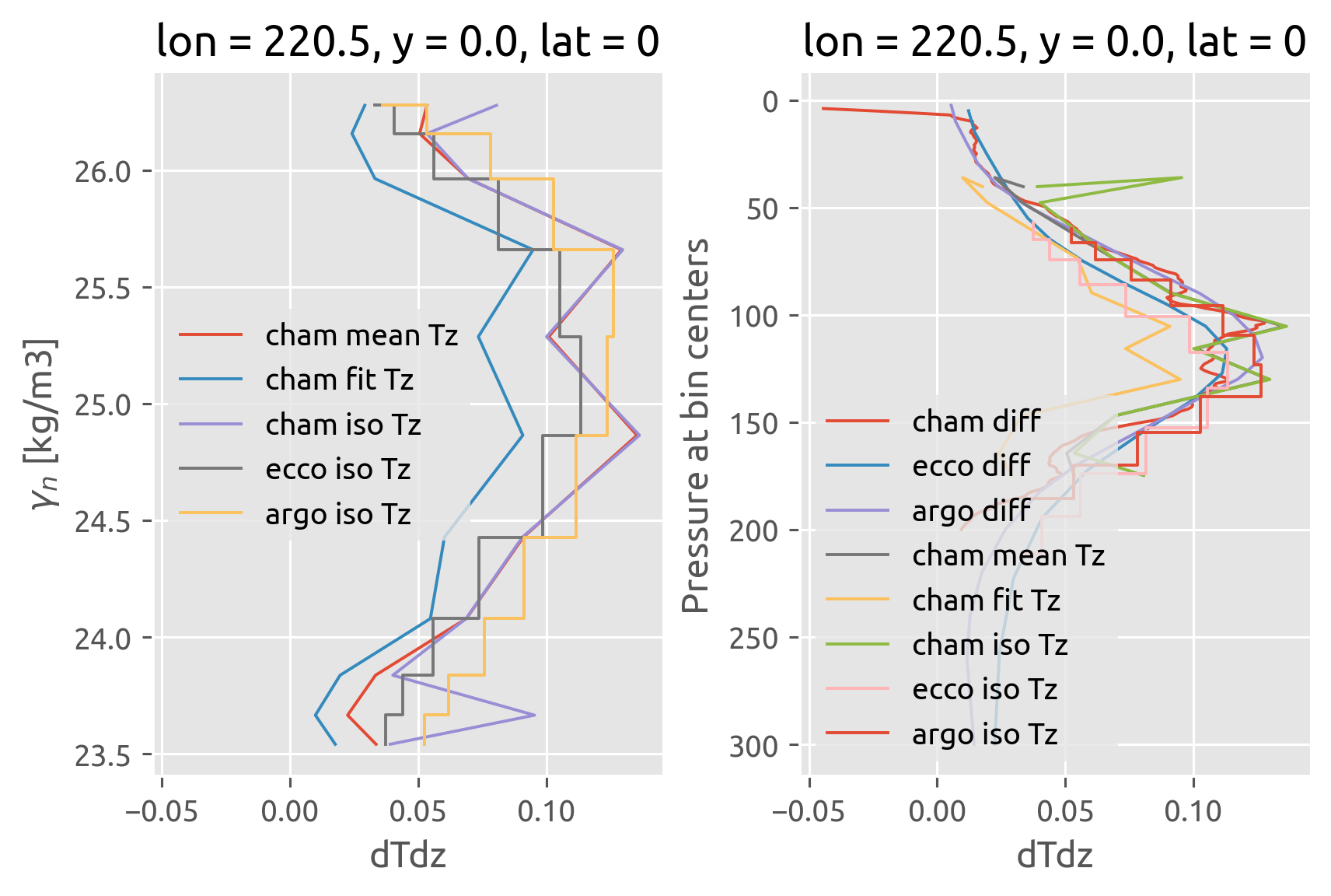
Cole et al (2015) estimate#
Let’s see what they used for variance, gradients at the same σ levels
cole = ed.read_cole()
cole
<xarray.Dataset>
Dimensions:                (lat: 131, lon: 360, pres: 101, scalar: 1, sigma: 96)
Coordinates:
  * lat                    (lat) float64 -65.0 -64.0 -63.0 ... 63.0 64.0 65.0
  * lon                    (lon) float64 1.5 2.5 3.5 4.5 ... 358.5 359.5 360.5
  * pres                   (pres) float64 0.0 20.0 40.0 ... 1.98e+03 2e+03
  * sigma                  (sigma) float64 20.0 20.1 20.2 ... 29.3 29.4 29.5
    start_year             (scalar) float64 2.005e+03
    end_year               (scalar) float64 2.015e+03
    mixing_efficiency      (scalar) float64 0.16
    minimum_points         (scalar) float64 15.0
    maximum_mixing_length  (scalar) float64 6e+05
Dimensions without coordinates: scalar
Data variables: (12/16)
    mixing_length_sig      (lat, lon, sigma) float64 ...
    salinity_mean_sig      (lat, lon, sigma) float64 ...
    salinity_std_sig       (lat, lon, sigma) float64 ...
    salinity_gradient_sig  (lat, lon, sigma) float64 ...
    depth_mean_sig         (lat, lon, sigma) float64 ...
    number_points_sig      (lat, lon, sigma) float64 ...
    ...                     ...
    density_mean_depth     (lat, lon, pres) float64 ...
    number_points          (lat, lon, pres) float64 ...
    velocity_std           (lat, lon, pres) float64 ...
    diffusivity            (lat, lon, pres) float64 nan nan nan ... nan nan nan
    process_date           (scalar) timedelta64[ns] 8 days 12:43:27.466400463
    diffusivity_first      (lat, lon) float64 nan nan nan nan ... nan nan nan
Attributes:
title: This dataset contains calculations related to the estimation of...- lat: 131
- lon: 360
- pres: 101
- scalar: 1
- sigma: 96
- lat(lat)float64-65.0 -64.0 -63.0 ... 64.0 65.0
- units :
- degrees north
- standard_name :
- latitude
array([-65., -64., -63., -62., -61., -60., -59., -58., -57., -56., -55., -54., -53., -52., -51., -50., -49., -48., -47., -46., -45., -44., -43., -42., -41., -40., -39., -38., -37., -36., -35., -34., -33., -32., -31., -30., -29., -28., -27., -26., -25., -24., -23., -22., -21., -20., -19., -18., -17., -16., -15., -14., -13., -12., -11., -10., -9., -8., -7., -6., -5., -4., -3., -2., -1., 0., 1., 2., 3., 4., 5., 6., 7., 8., 9., 10., 11., 12., 13., 14., 15., 16., 17., 18., 19., 20., 21., 22., 23., 24., 25., 26., 27., 28., 29., 30., 31., 32., 33., 34., 35., 36., 37., 38., 39., 40., 41., 42., 43., 44., 45., 46., 47., 48., 49., 50., 51., 52., 53., 54., 55., 56., 57., 58., 59., 60., 61., 62., 63., 64., 65.]) - lon(lon)float641.5 2.5 3.5 ... 358.5 359.5 360.5
- units :
- degrees east
- standard_name :
- longitude
array([ 1.5, 2.5, 3.5, ..., 358.5, 359.5, 360.5])
- pres(pres)float640.0 20.0 40.0 ... 1.98e+03 2e+03
- positive :
- down
array([ 0., 20., 40., 60., 80., 100., 120., 140., 160., 180., 200., 220., 240., 260., 280., 300., 320., 340., 360., 380., 400., 420., 440., 460., 480., 500., 520., 540., 560., 580., 600., 620., 640., 660., 680., 700., 720., 740., 760., 780., 800., 820., 840., 860., 880., 900., 920., 940., 960., 980., 1000., 1020., 1040., 1060., 1080., 1100., 1120., 1140., 1160., 1180., 1200., 1220., 1240., 1260., 1280., 1300., 1320., 1340., 1360., 1380., 1400., 1420., 1440., 1460., 1480., 1500., 1520., 1540., 1560., 1580., 1600., 1620., 1640., 1660., 1680., 1700., 1720., 1740., 1760., 1780., 1800., 1820., 1840., 1860., 1880., 1900., 1920., 1940., 1960., 1980., 2000.]) - sigma(sigma)float6420.0 20.1 20.2 ... 29.3 29.4 29.5
- positive :
- down
array([20. , 20.1, 20.2, 20.3, 20.4, 20.5, 20.6, 20.7, 20.8, 20.9, 21. , 21.1, 21.2, 21.3, 21.4, 21.5, 21.6, 21.7, 21.8, 21.9, 22. , 22.1, 22.2, 22.3, 22.4, 22.5, 22.6, 22.7, 22.8, 22.9, 23. , 23.1, 23.2, 23.3, 23.4, 23.5, 23.6, 23.7, 23.8, 23.9, 24. , 24.1, 24.2, 24.3, 24.4, 24.5, 24.6, 24.7, 24.8, 24.9, 25. , 25.1, 25.2, 25.3, 25.4, 25.5, 25.6, 25.7, 25.8, 25.9, 26. , 26.1, 26.2, 26.3, 26.4, 26.5, 26.6, 26.7, 26.8, 26.9, 27. , 27.1, 27.2, 27.3, 27.4, 27.5, 27.6, 27.7, 27.8, 27.9, 28. , 28.1, 28.2, 28.3, 28.4, 28.5, 28.6, 28.7, 28.8, 28.9, 29. , 29.1, 29.2, 29.3, 29.4, 29.5]) - start_year(scalar)float642.005e+03
- long_name :
- first year of data included in the calculations
array([2005.])
- end_year(scalar)float642.015e+03
- long_name :
- final year of data included in the calculations
array([2015.])
- mixing_efficiency(scalar)float640.16
- units :
- unitless
- long_name :
- mixing efficiency
array([0.16])
- minimum_points(scalar)float6415.0
- units :
- unitless
- long_name :
- minimum number of data points
array([15.])
- maximum_mixing_length(scalar)float646e+05
- units :
- meters
- long_name :
- maximum permitted mixing length
array([600000.])
- mixing_length_sig(lat, lon, sigma)float64...
- units :
- meters
- long_name :
- $λ$
- description :
- mixing length on density surfaces
[4527360 values with dtype=float64]
- salinity_mean_sig(lat, lon, sigma)float64...
- units :
- g/kg
- long_name :
- $S$
- description :
- mean salinity on density surfaces
[4527360 values with dtype=float64]
- salinity_std_sig(lat, lon, sigma)float64...
- units :
- g/kg
- long_name :
- $\sqrt{S'S'}$
- description :
- standard deviation of salinity on density surfaces
[4527360 values with dtype=float64]
- salinity_gradient_sig(lat, lon, sigma)float64...
- units :
- g/kg/m
- long_name :
- $|∇S|$
- description :
- horizontal gradient of mean salinity on density surfaces
[4527360 values with dtype=float64]
- depth_mean_sig(lat, lon, sigma)float64...
- units :
- meters
- long_name :
- mean depth of each density surface
[4527360 values with dtype=float64]
- number_points_sig(lat, lon, sigma)float64...
- units :
- unitless
- long_name :
- number of points in each bin on density surfaces
[4527360 values with dtype=float64]
- mixing_length(lat, lon, pres)float64...
- units :
- meters
- long_name :
- $λ$
- description :
- mixing length interpolated to depth surfaces
[4763160 values with dtype=float64]
- salinity_mean(lat, lon, pres)float64...
- units :
- g/kg
- long_name :
- $S$
- description :
- mean salinity interpolated to depth surfaces
[4763160 values with dtype=float64]
- salinity_std(lat, lon, pres)float64...
- units :
- g/kg
- long_name :
- $\sqrt{S'S'}$
- description :
- standard deviation of salinity interpolated to depth surfaces
[4763160 values with dtype=float64]
- salinity_gradient(lat, lon, pres)float64...
- units :
- g/kg/m
- long_name :
- $|∇S|$
- description :
- horizontal gradient of mean salinity interpolated to depth surfaces
[4763160 values with dtype=float64]
- density_mean_depth(lat, lon, pres)float64...
- units :
- meters
- long_name :
- mean density of each depth surface
[4763160 values with dtype=float64]
- number_points(lat, lon, pres)float64...
- units :
- unitless
- long_name :
- number of points in each bin interpolated to depth surfaces
[4763160 values with dtype=float64]
- velocity_std(lat, lon, pres)float64...
- units :
- m/s
- standard deviation of ECCO2 velocity on depth surfaces :
- m/s
[4763160 values with dtype=float64]
- diffusivity(lat, lon, pres)float64nan nan nan nan ... nan nan nan nan
- units :
- m^2/s
- long_name :
- $κ$
- description :
- eddy diffusivity on depth surfaces
array([[[nan, nan, ..., nan, nan], [nan, nan, ..., nan, nan], ..., [nan, nan, ..., nan, nan], [nan, nan, ..., nan, nan]], [[nan, nan, ..., nan, nan], [nan, nan, ..., nan, nan], ..., [nan, nan, ..., nan, nan], [nan, nan, ..., nan, nan]], ..., [[nan, nan, ..., nan, nan], [nan, nan, ..., nan, nan], ..., [nan, nan, ..., nan, nan], [nan, nan, ..., nan, nan]], [[nan, nan, ..., nan, nan], [nan, nan, ..., nan, nan], ..., [nan, nan, ..., nan, nan], [nan, nan, ..., nan, nan]]]) - process_date(scalar)timedelta64[ns]...
- long_name :
- date files were processed
array([737007466400463], dtype='timedelta64[ns]')
- diffusivity_first(lat, lon)float64nan nan nan nan ... nan nan nan nan
- units :
- m^2/s
- long_name :
- $κ$
- description :
- eddy diffusivity on depth surfaces
array([[nan, nan, nan, ..., nan, nan, nan],
       [nan, nan, nan, ..., nan, nan, nan],
       [nan, nan, nan, ..., nan, nan, nan],
       ...,
       [nan, nan, nan, ..., nan, nan, nan],
       [nan, nan, nan, ..., nan, nan, nan],
       [nan, nan, nan, ..., nan, nan, nan]])
- title :
- This dataset contains calculations related to the estimation of temperature-salinity variance and eddy diffusivity from the Argo data as described in Cole, S. T., C. Wortham, E. Kunze, and W. B. Owens, 2015: Eddy stirring and horizontal diffusivity from Argo float observations: Geographic and depth variability, Geophysical Research Letters, 42, 3989-3997.
def plot_pac(da):
    sigma_levels = [24.0, 25.0]
    fg = (
        da.sel(lat=slice(-10, 10), lon=slice(110, 360 - 70))
        .sel(sigma=sigma_levels, method="nearest")
        .plot(
            robust=True,
            # cbar_kwargs={"orientation": "horizontal"},
            col="sigma",
            col_wrap=2,
            aspect=1.4,
        )
    )
    for ax in fg.axes.flat:
        ax.plot(220, 0, marker="o", color="w")


plot_pac(cole.salinity_gradient_sig)
plot_pac(cole.salinity_std_sig)
plot_pac(cole.mixing_length_sig)
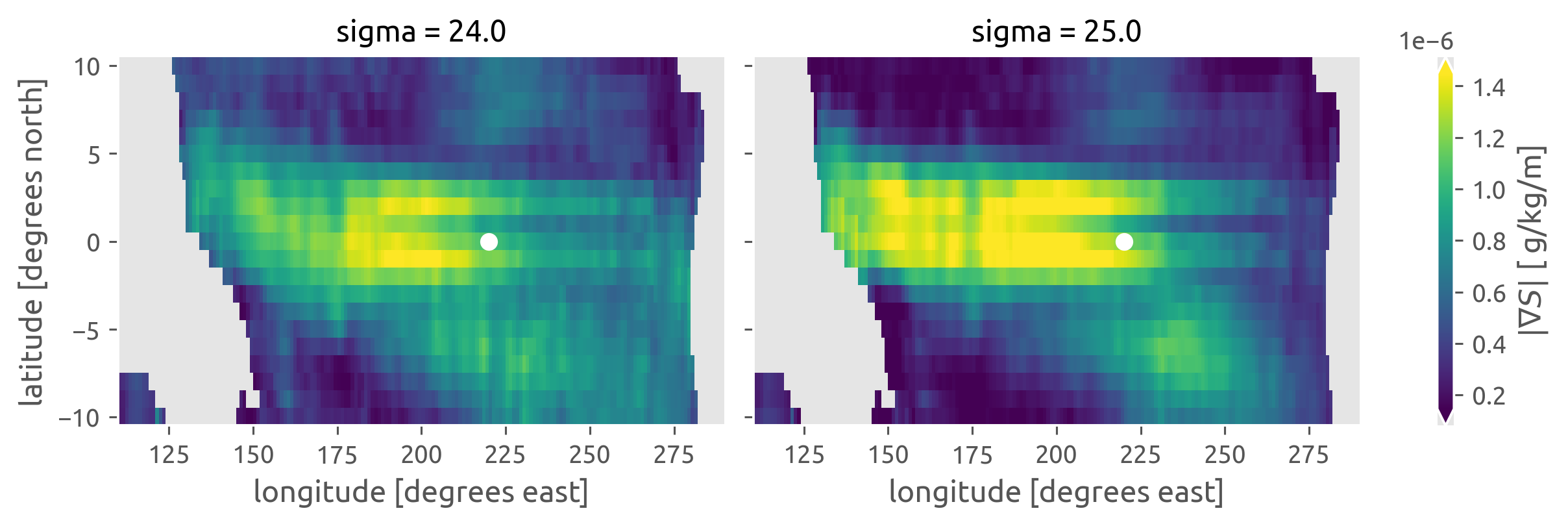
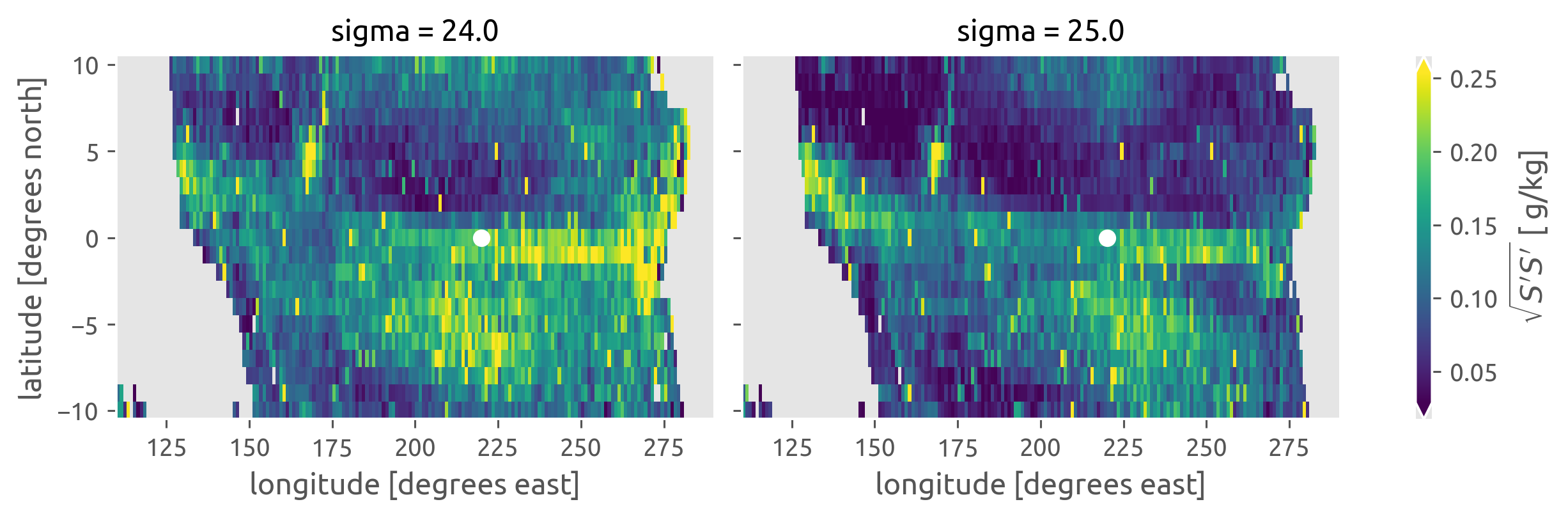
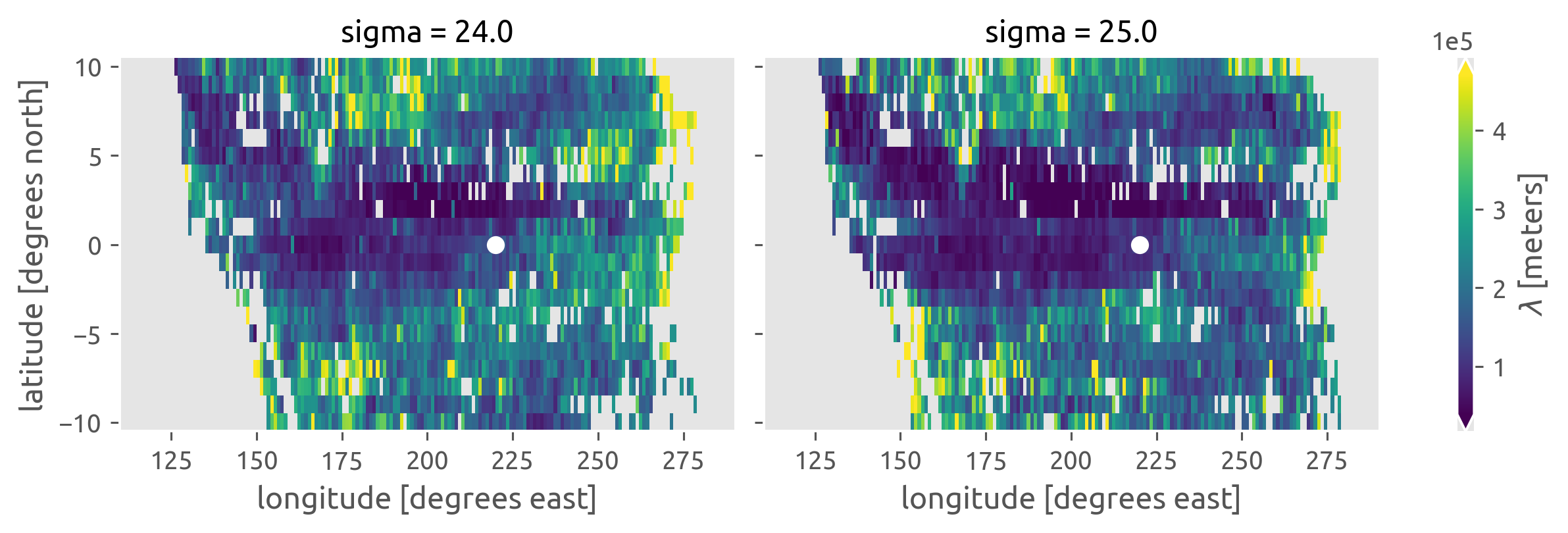
Profiles at (0, 140W)#
These look OK.
there is an order of magnitude larger \(\\sqrt{S'S'}\) between 40m and 150m than 250m-400m.
That matches a larger |∇S| in the same depth range
Next step: is the longitudinal gradient bigger than meridional gradient
import eddydiff as ed

ed.plot.plot_cole_profile(lat=0, lon=[221, 220, 219])
plt.gca().set_ylim(400, 0)
(400.0, 0.0)
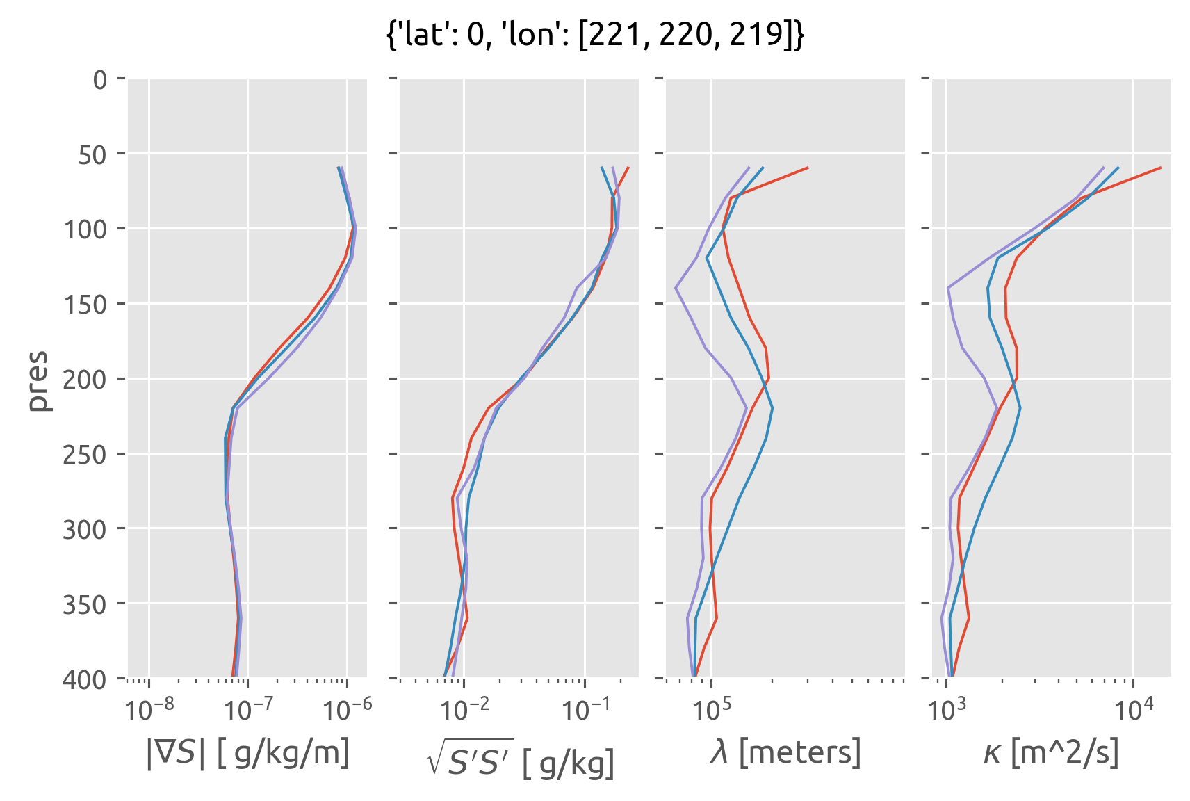
Todo:#
[ ] Seasonal cycle in iso Tz from ecco, argo?
[ ] look for stirring signal in Argo?
[ ]