χpods: EQUIX vs TAO

import cf_xarray
import dcpy
import distributed
import matplotlib as mpl
import matplotlib.pyplot as plt
import numpy as np
import pandas as pd
import pump

import eddydiff
import eddydiff as ed
import xarray as xr

xr.set_options(keep_attrs=True)

plt.style.use("bmh")
plt.rcParams["figure.dpi"] = 140
plt.rcParams["savefig.dpi"] = 200

eop = xr.open_dataset(
    "/home/deepak/datasets/microstructure/osu/equix/hourly_eop.nc"
).rename({"dTdz": "Tz"})
eop["salt"] = 35 * xr.ones_like(eop.theta)
eop["salt"].attrs = {"standard_name": "sea_water_salinity"}
eop["T"] = dcpy.eos.temp(eop.salt, eop.theta, eop.depth)
eop.coords["pres"] = dcpy.eos.pres(eop.depth, 0)
eop.coords["latitude"] = 0
eop.coords["longitude"] = -140
# eop["gamma_n"] = dcpy.oceans.neutral_density(eop)
# eop["pden"] = dcpy.eos.pden(eop.salt, eop.theta, 0)
eop.attrs["name"] = "EQUIX"

tao = xr.open_dataset("/home/deepak/datasets/microstructure/osu/equix/hourly_tao.nc")
tao.attrs["name"] = "TAO"
tao_eop = dcpy.util.slice_like(tao, eop.time).drop_sel(depth=[39, 84])
tao_eop

<xarray.Dataset>
Dimensions:  (depth: 5, time: 2692)
Coordinates:
  * time     (time) datetime64[ns] 2008-11-11T05:00:00 ... 2009-03-03T08:00:00
  * depth    (depth) int64 18 59 69 124 150
    unit     (depth) int64 313 325 319 327 321
Data variables:
    theta    (time, depth) float64 24.77 22.59 23.06 17.55 ... 23.33 18.66 15.89
    chi      (time, depth) float64 2.222e-07 3.024e-07 ... 2.655e-08 2.5e-07
    eps      (time, depth) float64 4.368e-07 5.899e-08 ... 3.465e-09 7.051e-09
    Kt       (time, depth) float64 0.008625 0.0001353 ... 6.772e-06 3.797e-06
    Jq       (time, depth) float64 98.86 17.36 1.291 ... 0.2414 1.153 2.633
    dTdz     (time, depth) float64 0.008565 0.03904 0.132 ... 0.06073 0.2235
Attributes:
    name:     TAO

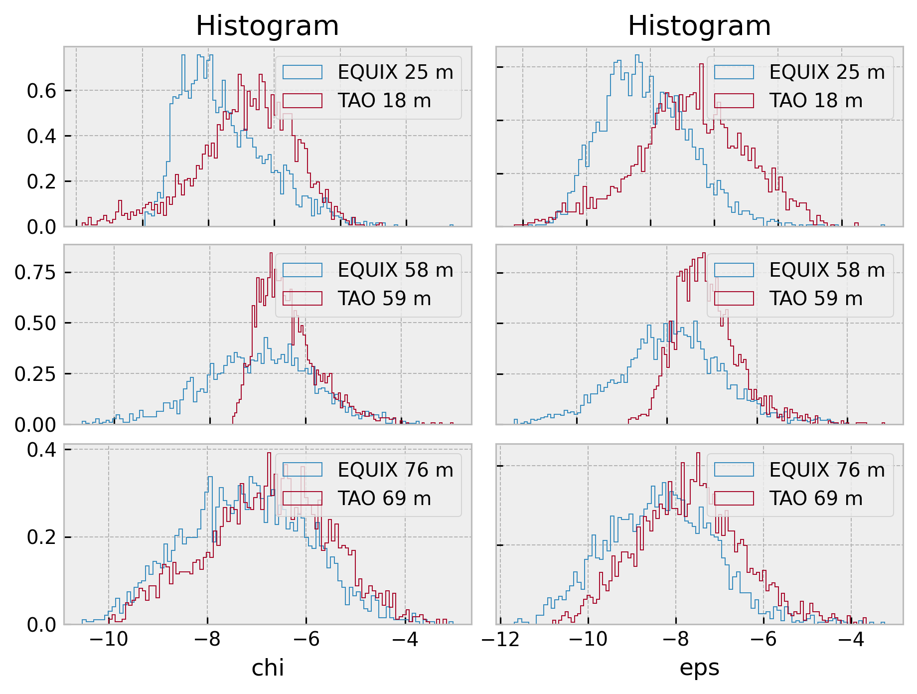
χ, ε distributions

TAO 59m looks weird

fg = dcpy.facetgrid.facetgrid([0, 1, 2], ["chi", "eps"], sharex=False, sharey=False)

for ds in [eop.sel(depth=[25, 58, 76]), tao_eop.sel(depth=[18, 59, 69])]:
    for idx, _ in enumerate(ds.depth):
        for var in fg.col_locs:
            np.log10(ds[var].isel(depth=idx)).plot.hist(
                ax=fg.axes_dict[idx][var],
                bins=100,
                histtype="step",
                label=f"{ds.attrs['name']} {ds.depth[idx].values} m",
                density=True,
            )
for ax in fg.axes.flat:
    ax.legend()

dcpy.plots.clean_axes(fg.axes)

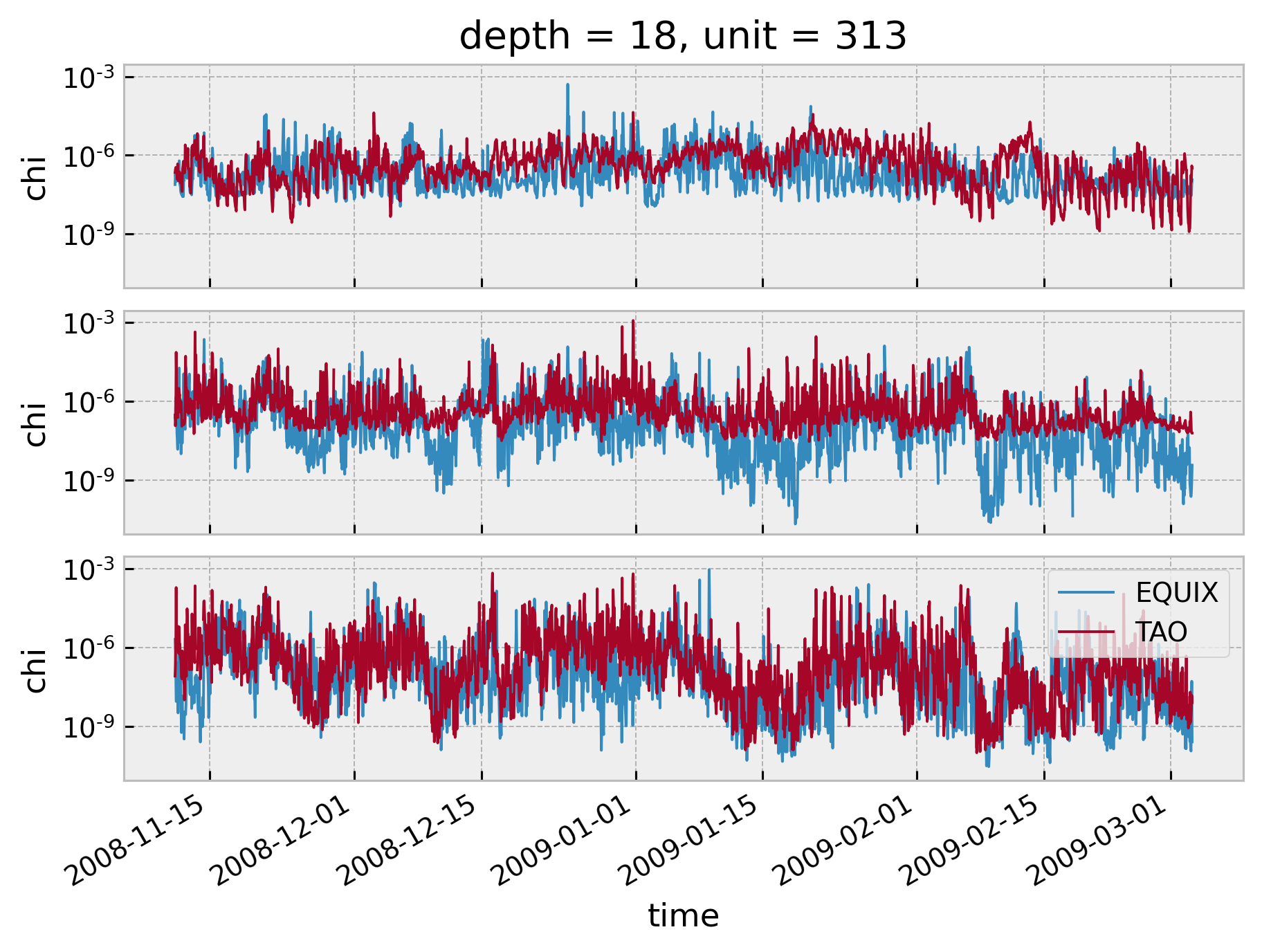
Time series

f, ax = plt.subplots(
    3, 1, squeeze=False, sharex=True, sharey=True, constrained_layout=True
)
for axis, depth in zip(ax.flat, [25, 58, 75]):
    kwargs = dict(yscale="log", x="time", lw=1, ax=axis)
    eop.sel(depth=depth, method="nearest").chi.plot(**kwargs)
    tao_eop.sel(depth=depth, method="nearest").chi.plot(**kwargs)
plt.legend(["EQUIX", "TAO"])
dcpy.plots.clean_axes(ax)

Time means

kwargs = dict(xscale="log", marker="o", ls="none", y="depth")
eop.chi.mean("time").cf.plot(**kwargs)
tao_eop.chi.mean("time").cf.plot(**kwargs)

[<matplotlib.lines.Line2D at 0x7f96051a83d0>]

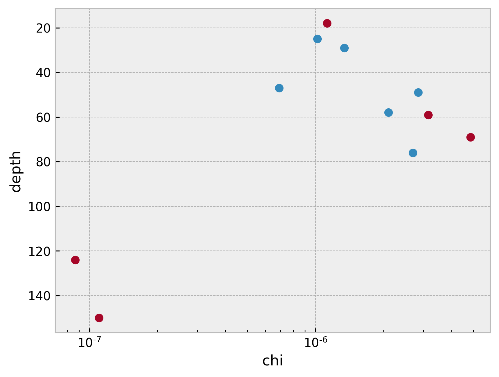
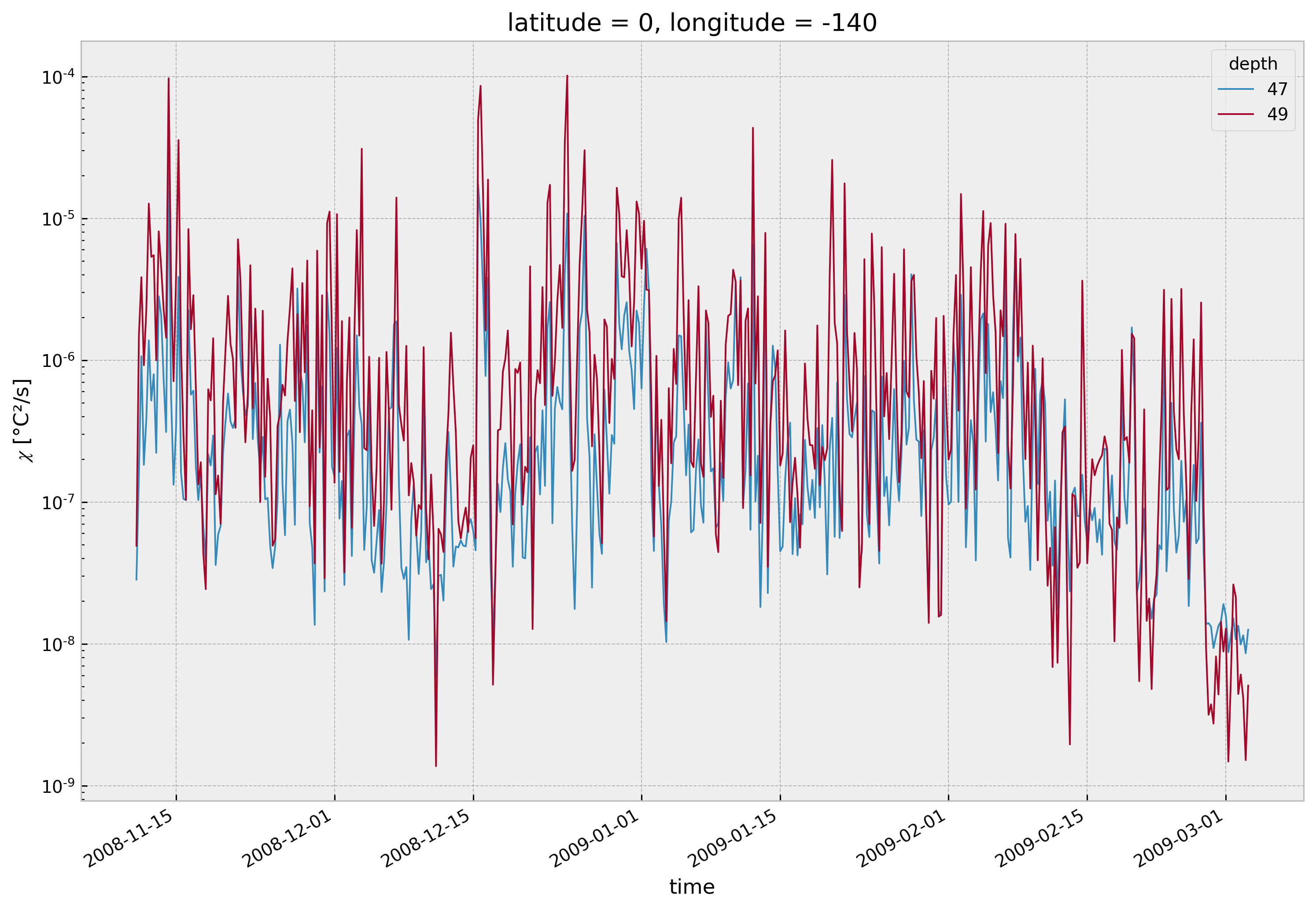
Compared with the surrounding points, it looks like EQUIX 47m is too low? Here’s a 12H average of 47m, 49m

eop.chi.sel(depth=[47, 49]).resample(time="6H").mean().plot.line(
    hue="depth", yscale="log", lw=1, size=8, aspect=1.6
)

[<matplotlib.lines.Line2D at 0x7f9606593df0>,
 <matplotlib.lines.Line2D at 0x7f96065b4790>]

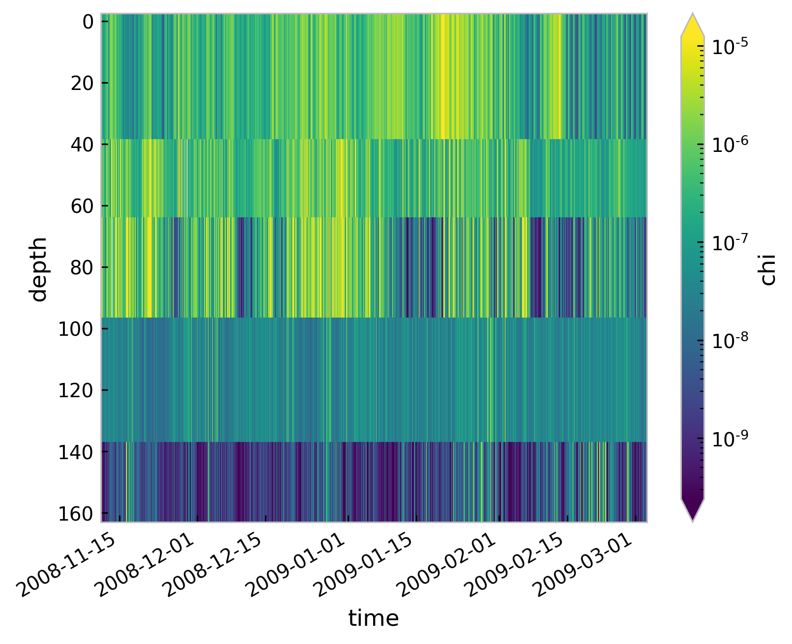
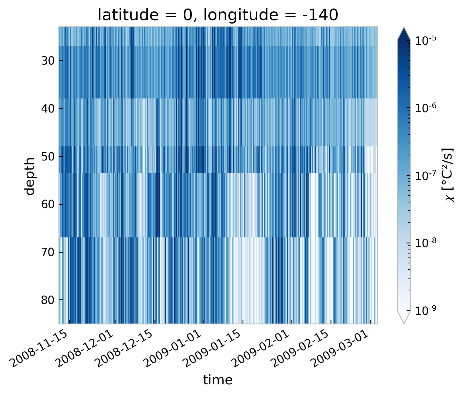
pcolor plots

tao_eop.chi.cf.plot(robust=True, norm=mpl.colors.LogNorm(1e-9, 1e-5), cmap=mpl.cm.Blues)

<matplotlib.collections.QuadMesh at 0x7f96143f6c70>

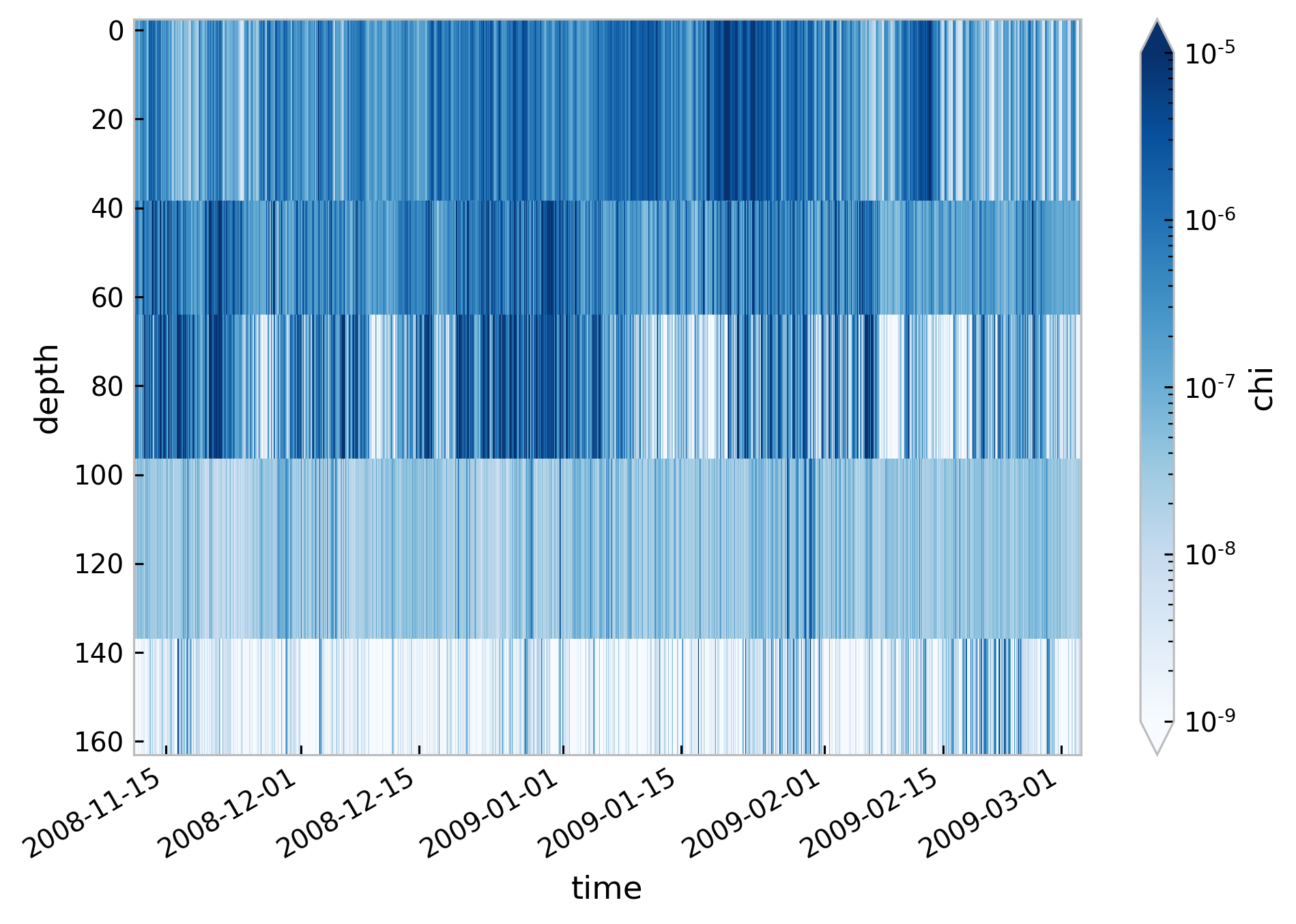
eop.chi.cf.plot(robust=True, norm=mpl.colors.LogNorm(1e-9, 1e-5), cmap=mpl.cm.Blues)

<matplotlib.collections.QuadMesh at 0x7f961571cd00>

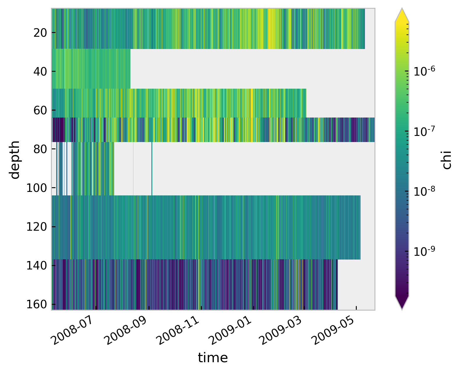
TAO Data availability

tao.chi.cf.plot(robust=True, norm=mpl.colors.LogNorm())
plt.figure()
tao_eop.chi.cf.plot(robust=True, norm=mpl.colors.LogNorm())

<matplotlib.collections.QuadMesh at 0x7f96145505e0>