Finescale Mixing Parametrizations: Development#
From Whalen et al (2012) Supplementary
QC:
All Argo float profiles with an ‘A’ quality rating (all real-time quality control tests passed) between June 2006 and December 2011 were selected.
The mixed layer was removed before implementing the parameterization since the mixed layer appears at a region of the high strain variance, and the parameterization treats all strain variance as internal waves, leading to an inaccurate estimate of the mixing. The same problem exists for other areas of low stratification near the surface (for example, mode water).
The variable temperature criterion (de Boyer Montegut et al., 2004) was therefore applied twice, once to remove the mixed layer, and a second time treating the bottom of the mixed layer as the surface.
Profiles with large spikes from any of the sensors were taken out of the dataset, and small salinity spikes needed to be removed from a subset of the profiles.
Steps:
Each profile containing 15 m resolution or better was divided into 200 m half-overlapping segments.
Segments were discarded if N² < 10−9 s−2 or if N² varied by more than 6 x 10⁻⁴ s−2, to remove sharp strain gradients not associated with internal waves.
We consider the vertical resolution of the segments since this could have an effect on the calculated dissipation rates. The majority of the segments had either 2 m or 10 m resolution, with similar mean ! (the mean 10 m resolution estimate above 500 m was only 10% larger), while the standard deviation of dissipation rate for 2 m data was 40% larger.
Whalen et al (2015):
To calculate the strain variance ⟨ξ²⟩, each segment was detrended, windowed using a sin² 10% taper, and spatially Fourier transformed to generate the spectrum Sstr for each segment. The spectrum is corrected for first differencing by dividing by the transfer function sinc² (kzDz/2p), where Dz is the vertical resolution of the segment. Argo data are either point measurements or averages over a depth interval, which is currently not identified in the metadata. Here, we correct for this whenever we know the sampling scheme of the profile by dividing by the same transfer function a second time [a correction not included in Whalen et al. (2012)]. This slightly raises the variances in the bin-averaged cases. The average increase in the dissipation rate for the Atlantic Ocean is a factor of 1.02, with a range of 1 to 2.6.
Strain \begin{equation} ξ_z = \frac{N² - N²_{fit}}{\bar{N²}} \end{equation}
Waterman et al (2014)
Segments were constructed both starting from the surface and the bottom, with near-surface values computed from the vertical segments defined starting from the surface, near-bottom values computed from the vertical segments defined starting from the bottom, and interior values computed from an average of top–down- and bottom–up-defined segments.
%load_ext watermark

import argopy
import cf_xarray as cfxr
import dask
import dcpy
import gsw
import matplotlib as mpl
import matplotlib.pyplot as plt
import mixsea
import numpy as np
import pandas as pd
import scipy
import scipy.integrate
import seawater as sw
from dcpy.finestructure import estimate_turb_segment
from scipy import signal
from scipy.io import loadmat

import xarray as xr

plt.style.use("bmh")
mpl.rcParams["figure.dpi"] = 140
mpl.rcParams["lines.linewidth"] = 1
dirname = "/home/deepak/datasets/finestructure/"

%watermark -iv
dask      : 2021.6.2
cf_xarray : 0.4.1.dev21+gab9dc66
scipy     : 1.5.3
eddydiff  : 0.1
pandas    : 1.2.3
seawater  : 3.3.4
dcpy      : 0.1
mixsea    : 0.1.0
xarray    : 0.17.1.dev3+g48378c4b1
numpy     : 1.20.2
argopy    : 0.1.7
gsw       : 3.4.0
matplotlib: 3.4.1
kunze = dcpy.oceans.read_kunze_2017_finestructure()
Check against Kunze & mixsea#
cruise = "317519930704"
cast = 19
kunze_cruise = kunze.groupby("cruise").get_group(cruise).query(f"drop == {cast}")

ctd = xr.open_mfdataset(f"{dirname}/../cchdo/{cruise}/*ctd.nc").load()
del ctd.attrs["comments"]

profile = ctd.query({"N_PROF": f"cast == {cast}"}).squeeze()
profile.ctd_salinity.attrs["standard_name"] = "sea_water_salinity"
profile["γ"] = dcpy.oceans.neutral_density(profile).reset_coords(drop=True)

# Polzin et al (2015) recommend sorting then calculating N2
initial_pressure = profile.pressure.reset_coords(drop=True)
profile = profile.sortby("γ")
profile["pressure"] = initial_pressure
profile = profile.swap_dims({"N_LEVELS": "pressure"})
profile = profile.isel(pressure=profile.pressure.notnull())

profile["N2"] = (
    "pressure",
    np.append(
        dcpy.eos.bfrq(
            profile.ctd_salinity,
            profile.ctd_temperature,
            profile.pressure,
            dim="pressure",
        )[0]
        # .interp(pressure_mid=profile.pressure.data)
        .data[1:],
        [np.nan, np.nan],
    ),
)

SA = gsw.SA_from_SP(
    profile.ctd_salinity, profile.pressure, profile.longitude, profile.latitude
)
CT = gsw.CT_from_t(SA, profile.ctd_temperature, profile.pressure)
N2gsw, p = gsw.Nsquared(SA, CT, profile.pressure, profile.latitude)
N2gsw = xr.DataArray(N2gsw, dims="pressure", coords={"pressure": p})

# profile["N2gsw"] = ("pressure", N2gsw.interp(pressure=profile.pressure.data).data)
profile["N2gsw"] = ("pressure", np.append(N2gsw, np.nan))

# Density variables σp, σθ, σ3, and γ_n and stratification N2 were then computed
profile["σθ"] = dcpy.eos.pden(
    profile.ctd_salinity, profile.ctd_temperature, profile.pressure, 0
)
profile["σ3"] = dcpy.eos.pden(
    profile.ctd_salinity, profile.ctd_temperature, profile.pressure, 3000
)

profile["N2θ"] = (
    -9.81
    / 1030
    * profile.σθ.cf.differentiate("sea_water_pressure", positive_upward=True)
)
profile["N23"] = (
    -9.81
    / 1030
    * profile.σ3.cf.differentiate("sea_water_pressure", positive_upward=True)
)
profile["N2γ"] = (
    -9.81
    / 1030
    * profile.γ.cf.differentiate("sea_water_pressure", positive_upward=True)
)

profile["pres"] = profile["pressure"]
Break up in to half overlapping segments
segmented = (
    profile.drop_vars("sample")
    .sel(pressure=slice(148, None))
    .rolling(pressure=128, min_periods=1)
    .construct(window_dim="segment", stride=64)
    .isel(pressure=slice(2, None))
)
segmented.coords["pres_mean"] = segmented.pres.mean("segment")
segmented["segment"] = np.arange(0, 2 * segmented.sizes["segment"], 2)
segmented
<xarray.Dataset>
Dimensions:             (pressure: 28, segment: 128)
Coordinates:
    latitude            float64 2.002
    longitude           float64 -25.2
    time                datetime64[ns] 1993-07-11T06:14:00
    expocode            object '3175MB93'
    station             object '16'
    cast                int8 19
    reference_pressure  int64 0
  * pressure            (pressure) float64 404.0 532.0 ... 3.732e+03 3.86e+03
    pres_mean           (pressure) float64 277.0 405.0 ... 3.605e+03 3.733e+03
  * segment             (segment) int64 0 2 4 6 8 10 ... 244 246 248 250 252 254
Data variables: (12/16)
    section_id          object 'AR21b'
    ctd_temperature     (pressure, segment) float32 14.0 13.87 ... 2.389 2.392
    ctd_temperature_qc  (pressure, segment) float32 2.0 2.0 2.0 ... 2.0 2.0 2.0
    ctd_salinity        (pressure, segment) float32 35.38 35.38 ... 34.89 34.89
    ctd_salinity_qc     (pressure, segment) float32 2.0 2.0 2.0 ... 2.0 2.0 2.0
    profile_type        object 'C'
    ...                  ...
    σθ                  (pressure, segment) float64 1.026e+03 ... 1.028e+03
    σ3                  (pressure, segment) float64 1.039e+03 ... 1.042e+03
    N2θ                 (pressure, segment) float64 0.0001127 ... 3.154e-06
    N23                 (pressure, segment) float64 0.0001539 ... 2.376e-06
    N2γ                 (pressure, segment) float32 0.0001192 ... 6.358e-08
    pres                (pressure, segment) float64 150.0 152.0 ... 3.86e+03
Attributes:
    Conventions:               CF-1.8 CCHDO-1.0
    cchdo_software_version:    hydro 1.0.1.2
    cchdo_parameters_version:  params 0.1.9
featureType: profile- pressure: 28
- segment: 128
- latitude()float642.002
- whp_name :
- LATITUDE
- standard_name :
- latitude
- units :
- degree_north
- C_format :
- %9.4f
- axis :
- Y
array(2.002)
- longitude()float64-25.2
- whp_name :
- LONGITUDE
- standard_name :
- longitude
- units :
- degree_east
- C_format :
- %9.4f
- axis :
- X
array(-25.202)
- time()datetime64[ns]1993-07-11T06:14:00
- standard_name :
- time
- axis :
- T
- whp_name :
- ['DATE', 'TIME']
- resolution :
- 0.000694
- geometry :
- geometry_container
array('1993-07-11T06:14:00.000000000', dtype='datetime64[ns]') - expocode()object'3175MB93'
- whp_name :
- EXPOCODE
- geometry :
- geometry_container
array('3175MB93', dtype=object) - station()object'16'
- whp_name :
- STNNBR
- geometry :
- geometry_container
array('16', dtype=object) - cast()int819
- whp_name :
- CASTNO
- geometry :
- geometry_container
array(19, dtype=int8)
- reference_pressure()int640
- units :
- dbar
array(0)
- pressure(pressure)float64404.0 532.0 ... 3.732e+03 3.86e+03
- whp_name :
- CTDPRS
- whp_unit :
- DBAR
- standard_name :
- sea_water_pressure
- units :
- dbar
- C_format :
- %9.1f
- axis :
- Z
- positive :
- down
array([ 404., 532., 660., 788., 916., 1044., 1172., 1300., 1428., 1556., 1684., 1812., 1940., 2068., 2196., 2324., 2452., 2580., 2708., 2836., 2964., 3092., 3220., 3348., 3476., 3604., 3732., 3860.]) - pres_mean(pressure)float64277.0 405.0 ... 3.605e+03 3.733e+03
array([ 277., 405., 533., 661., 789., 917., 1045., 1173., 1301., 1429., 1557., 1685., 1813., 1941., 2069., 2197., 2325., 2453., 2581., 2709., 2837., 2965., 3093., 3221., 3349., 3477., 3605., 3733.]) - segment(segment)int640 2 4 6 8 ... 246 248 250 252 254
array([  0,   2,   4,   6,   8,  10,  12,  14,  16,  18,  20,  22,  24,  26,
        28,  30,  32,  34,  36,  38,  40,  42,  44,  46,  48,  50,  52,  54,
        56,  58,  60,  62,  64,  66,  68,  70,  72,  74,  76,  78,  80,  82,
        84,  86,  88,  90,  92,  94,  96,  98, 100, 102, 104, 106, 108, 110,
       112, 114, 116, 118, 120, 122, 124, 126, 128, 130, 132, 134, 136, 138,
       140, 142, 144, 146, 148, 150, 152, 154, 156, 158, 160, 162, 164, 166,
       168, 170, 172, 174, 176, 178, 180, 182, 184, 186, 188, 190, 192, 194,
       196, 198, 200, 202, 204, 206, 208, 210, 212, 214, 216, 218, 220, 222,
       224, 226, 228, 230, 232, 234, 236, 238, 240, 242, 244, 246, 248, 250,
       252, 254])
- section_id()object'AR21b'
- whp_name :
- SECT_ID
- geometry :
- geometry_container
array('AR21b', dtype=object) - ctd_temperature(pressure, segment)float3214.0 13.87 13.84 ... 2.389 2.392
- whp_name :
- CTDTMP
- whp_unit :
- ITS-90
- standard_name :
- sea_water_temperature
- units :
- degC
- reference_scale :
- ITS-90
- C_format :
- %9.4f
- ancillary_variables :
- ctd_temperature_qc
array([[13.996, 13.869, 13.837, ..., 9.995, 9.941, 9.917], [12.363, 12.373, 12.367, ..., 5.956, 5.951, 5.944], [ 9.844, 9.903, 9.896, ..., 5.446, 5.441, 5.445], ..., [ 2.562, 2.559, 2.546, ..., 2.442, 2.451, 2.446], [ 2.487, 2.485, 2.48 , ..., 2.41 , 2.407, 2.41 ], [ 2.448, 2.448, 2.448, ..., 2.393, 2.389, 2.392]], dtype=float32) - ctd_temperature_qc(pressure, segment)float322.0 2.0 2.0 2.0 ... 2.0 2.0 2.0 2.0
- standard_name :
- status_flag
- flag_values :
- [0 1 2 3 4 5 6 7 9]
- flag_meanings :
- no_flag_assigned not_calibrated acceptable_measurement questionable_measurement bad_measurement not_reported interpolated_over_a_pressure_interval_larger_than_2_dbar despiked not_sampled
- conventions :
- WOCECTD - WOCE Quality Codes for CTD instrument measurements
array([[2., 2., 2., ..., 2., 2., 2.], [2., 2., 2., ..., 2., 2., 2.], [2., 2., 2., ..., 2., 2., 2.], ..., [2., 2., 2., ..., 2., 2., 2.], [2., 2., 2., ..., 2., 2., 2.], [2., 2., 2., ..., 2., 2., 2.]], dtype=float32) - ctd_salinity(pressure, segment)float3235.38 35.38 35.38 ... 34.89 34.89
- whp_name :
- CTDSAL
- whp_unit :
- PSS-78
- standard_name :
- sea_water_salinity
- units :
- 1
- reference_scale :
- PSS-78
- C_format :
- %9.4f
- ancillary_variables :
- ctd_salinity_qc
array([[35.379, 35.376, 35.379, ..., 34.906, 34.91 , 34.909], [35.192, 35.195, 35.194, ..., 34.532, 34.532, 34.532], [34.897, 34.911, 34.913, ..., 34.513, 34.513, 34.514], ..., [34.908, 34.907, 34.903, ..., 34.894, 34.897, 34.895], [34.899, 34.899, 34.898, ..., 34.892, 34.891, 34.892], [34.896, 34.896, 34.896, ..., 34.891, 34.889, 34.89 ]], dtype=float32) - ctd_salinity_qc(pressure, segment)float322.0 2.0 2.0 2.0 ... 2.0 2.0 2.0 2.0
- standard_name :
- status_flag
- flag_values :
- [0 1 2 3 4 5 6 7 9]
- flag_meanings :
- no_flag_assigned not_calibrated acceptable_measurement questionable_measurement bad_measurement not_reported interpolated_over_a_pressure_interval_larger_than_2_dbar despiked not_sampled
- conventions :
- WOCECTD - WOCE Quality Codes for CTD instrument measurements
array([[2., 2., 2., ..., 2., 2., 2.], [2., 2., 2., ..., 2., 2., 2.], [2., 2., 2., ..., 2., 2., 2.], ..., [2., 2., 2., ..., 2., 2., 2.], [2., 2., 2., ..., 2., 2., 2.], [2., 2., 2., ..., 2., 2., 2.]], dtype=float32) - profile_type()object'C'
array('C', dtype=object) - geometry_container()float64nan
- geometry_type :
- point
- node_coordinates :
- longitude latitude
array(nan)
- γ(pressure, segment)float3226.54 26.57 26.58 ... 28.1 28.1
- standard_name :
- neutral_density
- units :
- kg/m3
- long_name :
- $γ_n$
array([[26.541239, 26.566978, 26.576508, ..., 26.975796, 26.98863 , 26.992172], [26.74396 , 26.74418 , 26.74467 , ..., 27.325842, 27.326574, 27.327587], [26.996119, 26.996273, 26.999125, ..., 27.383345, 27.384216, 27.384338], ..., [28.085022, 28.085041, 28.08506 , ..., 28.096266, 28.09627 , 28.09627 ], [28.091358, 28.09164 , 28.091845, ..., 28.100817, 28.100845, 28.100847], [28.096346, 28.096376, 28.096405, ..., 28.103762, 28.103916, 28.10394 ]], dtype=float32) - N2(pressure, segment)float644.377e-05 1.483e-05 ... -2.582e-06
array([[ 4.37680791e-05, 1.48312208e-05, 4.73837291e-06, ..., 1.68648353e-05, 1.74886791e-05, 2.18544961e-06], [ 2.29621811e-06, 1.43986530e-06, 7.41253409e-06, ..., 4.73582718e-06, 3.19693034e-07, 5.39240079e-06], [ 1.35492023e-05, 3.17093601e-06, 2.64434973e-06, ..., 1.27107685e-06, 7.62273382e-07, 1.15745656e-07], ..., [-4.07379801e-06, -2.90621147e-07, 1.89295484e-06, ..., -2.99651830e-06, 2.17962714e-06, 1.83226394e-07], [ 5.63791173e-07, 1.39833071e-06, -2.37656554e-07, ..., 1.33141164e-06, 1.88266167e-07, -9.53537987e-07], [ 1.83318164e-07, -1.81904599e-07, 1.36290282e-06, ..., 1.29424653e-06, 2.96984115e-06, -2.58174075e-06]]) - N2gsw(pressure, segment)float640.0001185 4.387e-05 ... 3.051e-06
array([[ 1.18506609e-04, 4.38686551e-05, 1.48307925e-05, ..., 6.11738335e-05, 1.69535409e-05, 1.74934893e-05], [ 1.84632101e-06, 2.34153488e-06, 1.28642565e-06, ..., 3.47290790e-06, 4.79624301e-06, 3.59136330e-07], [ 2.32988969e-06, 1.36381534e-05, 3.19817653e-06, ..., 3.39959423e-06, 1.31906143e-06, 8.04467609e-07], ..., [-1.09324590e-06, -4.13324217e-06, -2.85213424e-07, ..., 3.81394030e-06, -3.04332688e-06, 2.23381175e-06], [ 1.82940548e-06, 5.86523661e-07, 1.43137761e-06, ..., -9.62941362e-07, 1.36803456e-06, 2.03074796e-07], [ 1.97803878e-07, 1.97899500e-07, -1.71548886e-07, ..., -3.74424645e-06, 1.33841261e-06, 3.05149195e-06]]) - σθ(pressure, segment)float641.026e+03 1.027e+03 ... 1.028e+03
- standard_name :
- sea_water_potential_density
- units :
- kg/m3
array([[1026.48554736, 1026.50997682, 1026.51906077, ..., 1026.88743526, 1026.89977443, 1026.90310077], [1026.6753066 , 1026.67574139, 1026.67618586, ..., 1027.1942568 , 1027.19490737, 1027.19580866], [1026.90609426, 1026.90711293, 1026.90989939, ..., 1027.24312459, 1027.24374314, 1027.24407838], ..., [1027.87475613, 1027.87421834, 1027.87209017, ..., 1027.87545326, 1027.87715653, 1027.87597129], [1027.87476483, 1027.87494355, 1027.87456259, ..., 1027.87753667, 1027.8769906 , 1027.8775727 ], [1027.87663072, 1027.87664865, 1027.87666659, ..., 1027.87923339, 1027.87796337, 1027.87854702]]) - σ3(pressure, segment)float641.039e+03 1.039e+03 ... 1.042e+03
- standard_name :
- sea_water_potential_density
- units :
- kg/m3
array([[1039.31503359, 1039.34649341, 1039.35729086, ..., 1039.96225127, 1039.9778912 , 1039.98275335], [1039.60123286, 1039.6010459 , 1039.6018722 , ..., 1040.5475624 , 1040.54858224, 1040.54999552], [1039.9905846 , 1039.98762847, 1039.99082545, ..., 1040.63432969, 1040.63532335, 1040.63535899], ..., [1041.49449975, 1041.49423876, 1041.49324502, ..., 1041.50715796, 1041.50809795, 1041.50737223], [1041.50173211, 1041.50208578, 1041.5021399 , ..., 1041.51295465, 1041.51268711, 1041.51302664], [1041.50786789, 1041.50790355, 1041.50793922, ..., 1041.51717566, 1041.51628729, 1041.51662858]]) - N2θ(pressure, segment)float640.0001127 7.98e-05 ... 3.154e-06
array([[ 1.12710321e-04, 7.97977083e-05, 2.83347463e-05, ..., 8.18469556e-05, 3.73006346e-05, 1.50479430e-05], [ 3.46432094e-06, 2.09357845e-06, -8.77930767e-07, ..., 7.76676329e-06, 3.69508851e-06, 2.10305380e-06], [ 9.55322223e-06, 9.06027533e-06, 7.74120007e-06, ..., 2.66161535e-06, 2.27105173e-06, 1.13356525e-06], ..., [ 8.50945482e-08, -6.34782784e-06, -6.15613438e-06, ..., 3.13995285e-06, 1.23344261e-06, -1.25199511e-06], [-6.79401345e-07, -4.81531029e-07, 4.67834139e-07, ..., -1.25734817e-06, 8.57890363e-08, 1.42892624e-06], [ 1.61285432e-06, 8.54196699e-08, -1.06259803e-06, ..., 2.73536830e-07, -1.63429040e-06, 3.15388149e-06]]) - N23(pressure, segment)float640.0001539 0.0001006 ... 2.376e-06
array([[ 1.53909538e-04, 1.00617441e-04, 4.53640376e-05, ..., 1.05203257e-04, 4.88168563e-05, 3.02238481e-05], [ 3.17135818e-07, 1.52231641e-06, 2.70809179e-05, ..., 9.92620414e-06, 5.79342485e-06, 4.42562600e-06], [ 1.16079768e-05, 5.73495960e-07, 1.20843578e-05, ..., 4.27524776e-06, 2.45081752e-06, 6.23508882e-07], ..., [ 1.67063852e-07, -2.98761426e-06, -2.60841705e-06, ..., 2.36000997e-06, 5.10181958e-07, -5.47805691e-07], [ 5.85657835e-07, 9.70984896e-07, 9.25997557e-07, ..., -5.51342749e-07, 1.71415255e-07, 8.94173251e-07], [ 1.26511801e-06, 1.69853917e-07, -1.70633720e-07, ..., 5.48361282e-07, -1.30264641e-06, 2.37552127e-06]]) - N2γ(pressure, segment)float320.0001192 8.398e-05 ... 6.358e-08
array([[1.1915604e-04, 8.3977371e-05, 3.0650765e-05, ..., 8.5385247e-05, 3.8993549e-05, 1.7830034e-05], [2.6068362e-06, 1.6939895e-06, 2.8066636e-06, ..., 8.2610368e-06, 4.1554968e-06, 2.5977533e-06], [9.7642824e-06, 7.1574459e-06, 8.7515218e-06, ..., 3.4561019e-06, 2.3661355e-06, 5.4044170e-07], ..., [6.8122901e-08, 9.0830532e-08, 6.3581375e-08, ..., 3.7240520e-07, 9.0830534e-09, 1.8166106e-07], [9.1284687e-07, 1.1580893e-06, 6.7668748e-07, ..., 1.4078732e-07, 7.2664427e-08, 7.2664427e-08], [2.5432550e-07, 1.4078732e-07, 4.1782044e-07, ..., 3.7240520e-07, 4.2236198e-07, 6.3581375e-08]], dtype=float32) - pres(pressure, segment)float64150.0 152.0 ... 3.858e+03 3.86e+03
- whp_name :
- CTDPRS
- whp_unit :
- DBAR
- standard_name :
- sea_water_pressure
- units :
- dbar
- C_format :
- %9.1f
- axis :
- Z
- positive :
- down
array([[ 150.,  152.,  154., ...,  400.,  402.,  404.],
       [ 278.,  280.,  282., ...,  528.,  530.,  532.],
       [ 406.,  408.,  410., ...,  656.,  658.,  660.],
       ...,
       [3350., 3352., 3354., ..., 3600., 3602., 3604.],
       [3478., 3480., 3482., ..., 3728., 3730., 3732.],
       [3606., 3608., 3610., ..., 3856., 3858., 3860.]])
- Conventions :
- CF-1.8 CCHDO-1.0
- cchdo_software_version :
- hydro 1.0.1.2
- cchdo_parameters_version :
- params 0.1.9
- featureType :
- profile
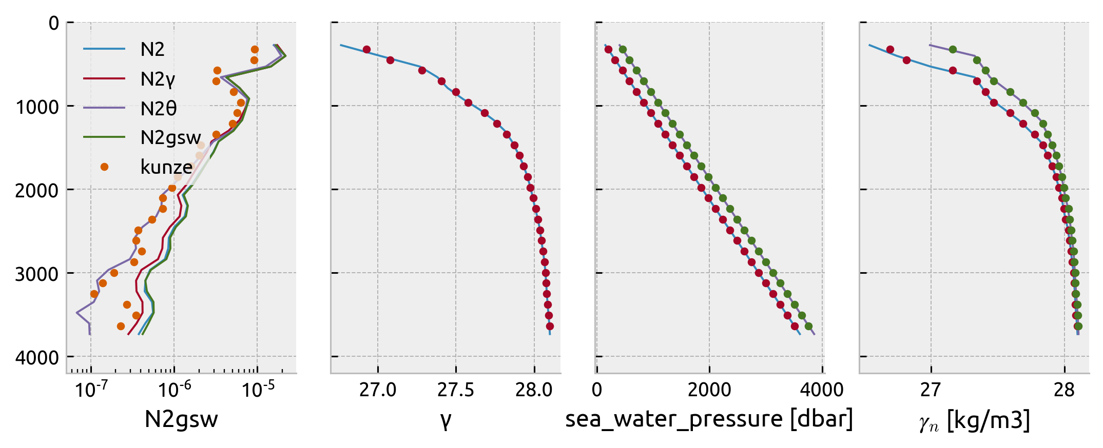
Compare N² estimates:#
Kunze seems to be using something like N² using pot temp referenced to surface! What!
f, ax = plt.subplots(1, 4, sharey=True)

axx = ax.ravel()
for var in ["N2", "N2γ", "N2θ", "N2gsw"]:
    segmented[var].mean("segment").plot(
        y="pres_mean", ax=axx[0], label=var, xscale="log"
    )
# (segmented.N2_γ.mean("segment")).plot(y="pres_mean", ax=axx[0], xscale="log")
axx[0].plot(kunze_cruise.N2, -1 * kunze_cruise.z_mean, ".", label="kunze")
# mod.N2mean.plot(hue="kind", ax=axx[0], y="depth_bin")
axx[0].legend()

segmented.γ.mean("segment").plot(y="pres_mean", ax=axx[1])
axx[1].plot(kunze_cruise.γ_mean, -1 * kunze_cruise.z_mean, ".")

segmented.pres.isel(segment=0).plot(y="pres_mean", ax=axx[2])
axx[2].plot(-1 * kunze_cruise.z_i, -1 * kunze_cruise.z_mean, ".")
segmented.pres.isel(segment=-1).plot(y="pres_mean", ax=axx[2])
axx[2].plot(-1 * kunze_cruise.z_f, -1 * kunze_cruise.z_mean, ".")

segmented.γ.isel(segment=0).plot(y="pres_mean", ax=axx[3])
axx[3].plot(kunze_cruise.γ_i, -1 * kunze_cruise.z_mean, ".")
segmented.γ.isel(segment=-1).plot(y="pres_mean", ax=axx[3])
axx[3].plot(kunze_cruise.γ_f, -1 * kunze_cruise.z_mean, ".")

[aa.set_title("") for aa in axx]
[aa.set_ylabel("") for aa in axx]
plt.tight_layout()
axx[0].set_ylim([4200, 0])
f.set_size_inches((8, 3))
from dcpy.finestructure import do_mixsea_shearstrain, estimate_turb_segment
results = xr.Dataset(coords={"pressure": segmented.pres_mean})
for var in ["K", "ε", "ξvar", "ξvargm"]:
results[var] = xr.full_like(segmented.pressure, np.nan)
for idx in range(segmented.sizes["pressure"]):
seg = segmented.isel(pressure=idx, drop=True).set_coords("pres")
(
results.K.data[idx],
results.ε.data[idx],
results.ξvar.data[idx],
results.ξvargm.data[idx],
_,
_,
) = estimate_turb_segment(
seg.cf["sea_water_pressure"].data + 1,
seg.N2.data,
seg.cf["latitude"].item(),
crit="kunze",
)
print("------------ mixsea")
mod = do_mixsea_shearstrain(
profile.isel(pressure=slice(148, None)), segmented.pres_mean.data
)
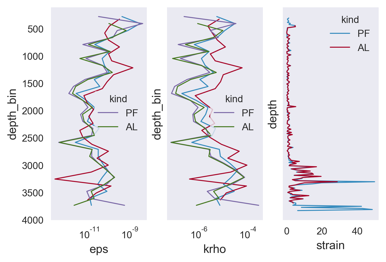
f, ax = plt.subplots(1, 3, sharey=True)
results.ε.cf.plot(xscale="log", ax=ax[0])
ax[0].plot(kunze_cruise.ε, -1 * kunze_cruise.z_mean)
mod.eps.plot(hue="kind", ax=ax[0], y="depth_bin")
results.K.cf.plot(xscale="log", ax=ax[1])
ax[1].plot(kunze_cruise.K, -1 * kunze_cruise.z_mean)
mod.krho.plot(hue="kind", ax=ax[1], y="depth_bin")
mod.strain.coarsen(depth=10, boundary="trim").var().plot(
hue="kind", ax=ax[2], y="depth"
)
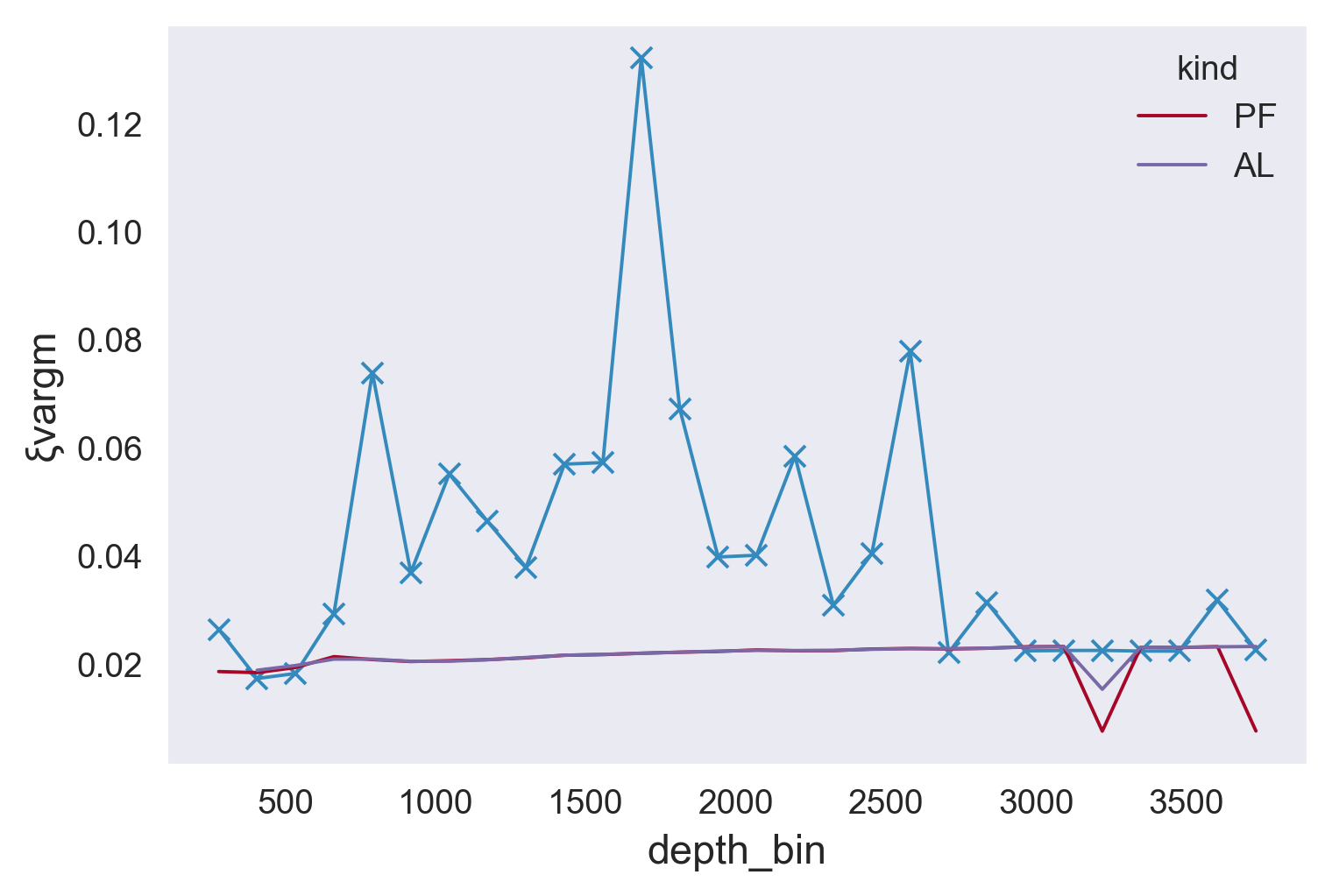
plt.figure()
(results.ξvargm).plot(marker="x")
(mod.ξvargm).plot(hue="kind")
plt.figure()
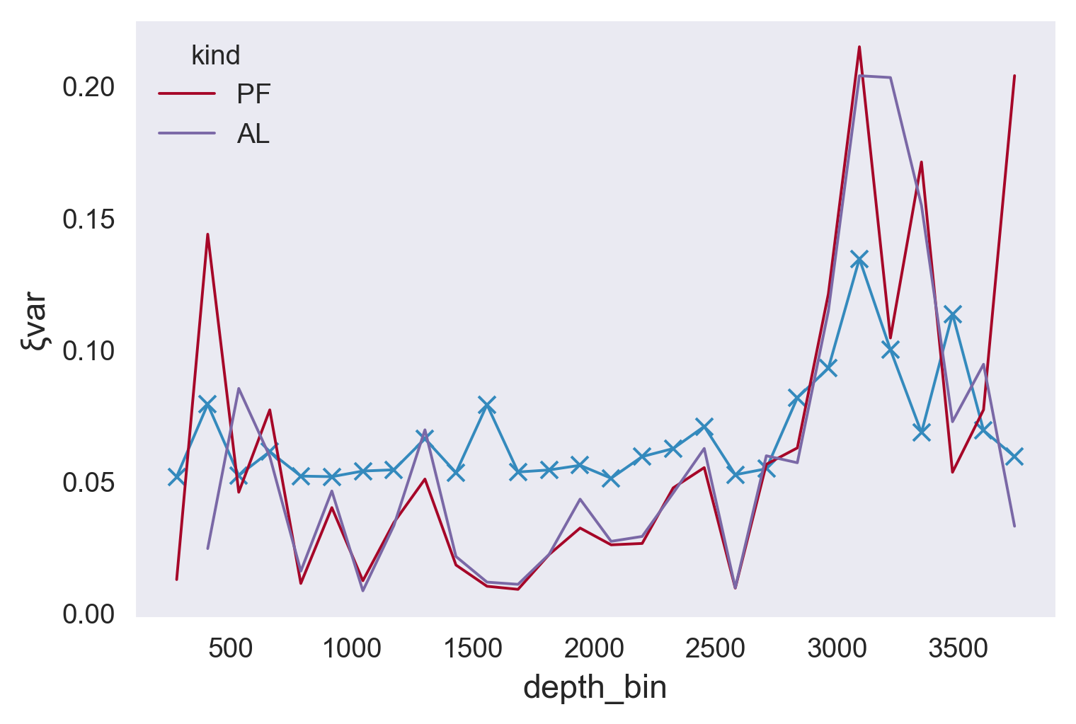
(results.ξvar).plot(marker="x")
mod.ξvar.plot(hue="kind")
# estimate_turb_segment(segmented.isel(pressure=5, drop=True).set_coords("pres"), debug=True)#
------------ mixsea
/home/deepak/miniconda3/envs/dcpy/lib/python3.8/site-packages/numpy/core/fromnumeric.py:3419: RuntimeWarning: Mean of empty slice.
  return _methods._mean(a, axis=axis, dtype=dtype,
/home/deepak/miniconda3/envs/dcpy/lib/python3.8/site-packages/numpy/core/_methods.py:188: RuntimeWarning: invalid value encountered in double_scalars
  ret = ret.dtype.type(ret / rcount)
/home/deepak/work/python/xarray/xarray/core/nputils.py:152: RuntimeWarning: Degrees of freedom <= 0 for slice.
  result = getattr(npmodule, name)(values, axis=axis, **kwargs)
[<matplotlib.lines.Line2D at 0x7f0b5454e5b0>,
 <matplotlib.lines.Line2D at 0x7f0b5454e5e0>]
segmented.ctd_temperature.polyfit("segment", deg=1)
<xarray.Dataset>
Dimensions:               (degree: 2, pressure: 28)
Coordinates:
  * degree                (degree) int64 1 0
  * pressure              (pressure) float64 404.0 532.0 ... 3.732e+03 3.86e+03
Data variables:
polyfit_coefficients (degree, pressure) float64 -0.01245 -0.02878 ... 2.438- degree: 2
- pressure: 28
- degree(degree)int641 0
array([1, 0])
- pressure(pressure)float64404.0 532.0 ... 3.732e+03 3.86e+03
array([ 404.,  532.,  660.,  788.,  916., 1044., 1172., 1300., 1428., 1556.,
       1684., 1812., 1940., 2068., 2196., 2324., 2452., 2580., 2708., 2836.,
       2964., 3092., 3220., 3348., 3476., 3604., 3732., 3860.])
- polyfit_coefficients(degree, pressure)float64-0.01245 -0.02878 ... 2.484 2.438
array([[-1.24475460e-02, -2.87833760e-02, -1.64239307e-02,
        -3.57453125e-03, -2.82412778e-03, -1.92586315e-03,
        -2.61825670e-04, -2.82020898e-04, -6.58043920e-04,
        -1.21086191e-03, -1.85757388e-03, -1.73998303e-03,
        -1.43382047e-03, -1.33599621e-03, -9.84765489e-04,
        -1.14968645e-03, -1.30315667e-03, -8.46881578e-04,
        -6.48393129e-04, -7.41518031e-04, -6.63791985e-04,
        -3.29986063e-04, -2.67809558e-04, -2.71622176e-04,
        -4.02151254e-04, -4.94131676e-04, -3.06328240e-04,
        -2.08798983e-04],
       [ 1.37042759e+01,  1.31632544e+01,  8.75928452e+00,
         5.93109046e+00,  5.42452359e+00,  4.99264712e+00,
         4.63026746e+00,  4.60402755e+00,  4.59796220e+00,
         4.55267008e+00,  4.44402908e+00,  4.20054036e+00,
         3.95786083e+00,  3.76781215e+00,  3.57185429e+00,
         3.45465082e+00,  3.31391497e+00,  3.11432740e+00,
         2.99384594e+00,  2.91758687e+00,  2.81716098e+00,
         2.71107232e+00,  2.66522277e+00,  2.63060540e+00,
         2.60490915e+00,  2.55980161e+00,  2.48366934e+00,
         2.43831436e+00]])
Compare to mixsea & Sensitivity studies#
The real difference is because they do some funny interpolating of the spectrum that I do not understand: https://github.com/modscripps/mixsea/blob/2c1a27b5b18d8b28f1af17e6d7dbe0f505ef78d8/mixsea/helpers.py#L169-L178
If I comment out that interp step, spectra agree exactly.
Sensitivity
The problem is that the cutoff wavenumber chosen depends a lot on spectrum; and then that determines how much of the GM spectrum is integrated. Taken together you get a lot of sensitivity just from that :/
Method of choosing the cutoff wavenumber matters too
So does Rω or shear-strain ratio.
I think part of the disagreement is also because the mixsea thing isn’t using the same bins
seg = segmented.isel(pressure=9)
dp = 2
N2 = seg.N2gsw
seg["N2fit"] = (
seg.N2.dims,
np.polyval(np.polyfit(seg.segment, N2, deg=2), seg.segment),
)
ξ = (N2 - seg.N2fit) / seg.N2fit.mean()
N = np.sqrt(seg.N2fit.mean())
_, _, Ptot, m = mixsea.helpers.psd(ξ.data, dp, ffttype="t", window="hamming")
npts = len(ξ.data)
window = signal.get_window("hann", npts)
window /= np.sqrt(np.sum(window**2) / len(window))
kz, psd = signal.periodogram(
ξ.data, window="hamming", fs=2 * np.pi / dp, detrend="linear", scaling="density"
)
# psd /= np.sinc(kz * dp / 2 / np.pi) ** 2
strain = mixsea.shearstrain.strain_polynomial_fits(
-1 * gsw.z_from_p(seg.pres_mean.data - 127 + seg.segment.data, seg.latitude.data),
seg.ctd_temperature.data,
seg.ctd_salinity.data,
seg.longitude.data,
seg.latitude.data,
# bin_width=64,
depth_bin=[seg.pres_mean.data],
window_size=350,
)
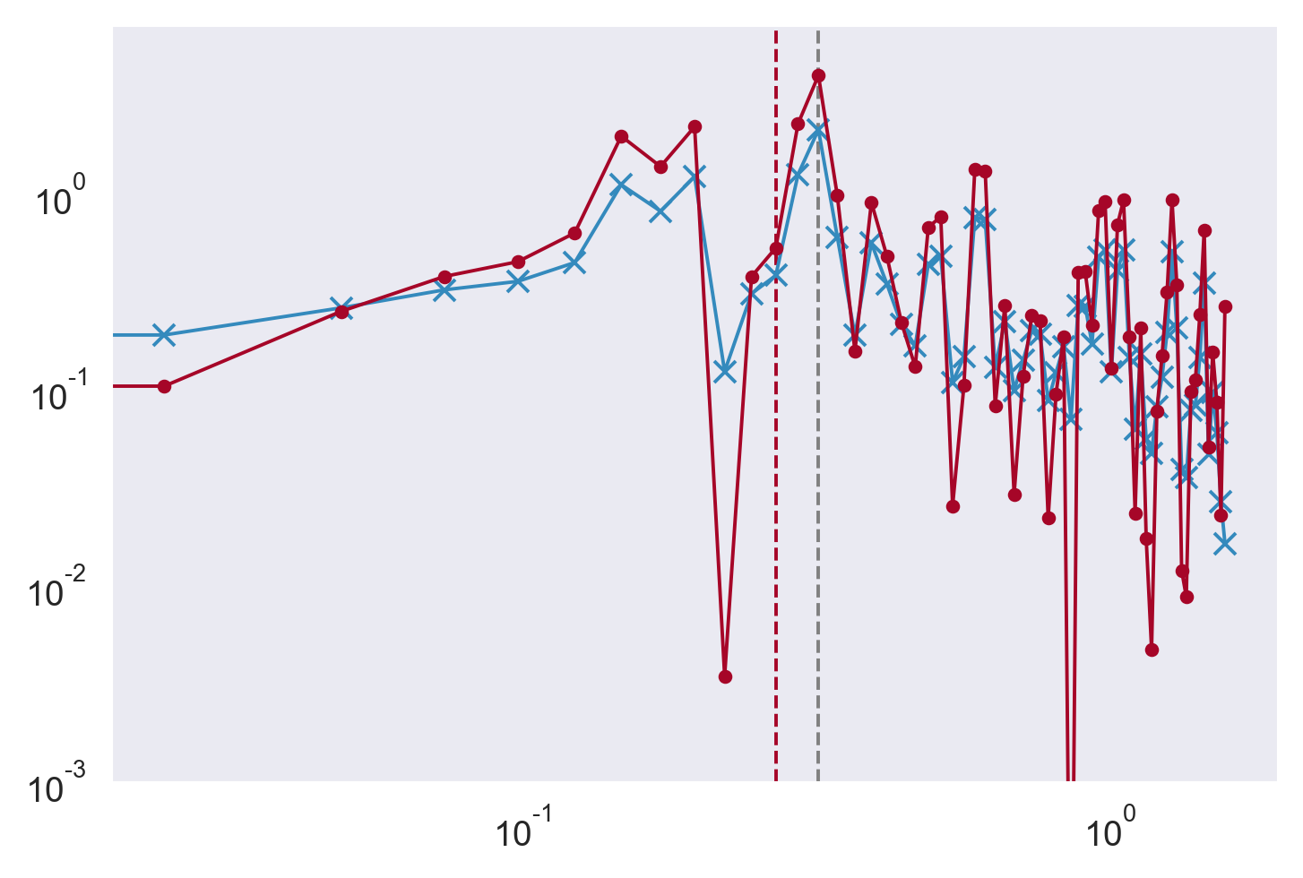
plt.loglog(m, Ptot, "x-")
ax = plt.gca()
imix, _ = mixsea.shearstrain.find_cutoff_wavenumber(Ptot, m, 0.22)
dcpy.plots.linex(m[imix[-1]])
print(
np.trapz(np.real(Ptot[imix]), m[imix]),
mixsea.shearstrain.gm_strain_variance(m, imix, np.sqrt(strain[0]["N2mean"]))[0],
)
plt.loglog(kz, psd, ".-")
imix, _ = mixsea.shearstrain.find_cutoff_wavenumber(psd, kz, 0.22)
dcpy.plots.linex(kz[imix[-1]], color="C1")
print(
np.trapz(psd[imix], kz[imix]),
mixsea.shearstrain.gm_strain_variance(kz, imix, N.data)[0],
)
plt.ylim([1e-3, None])
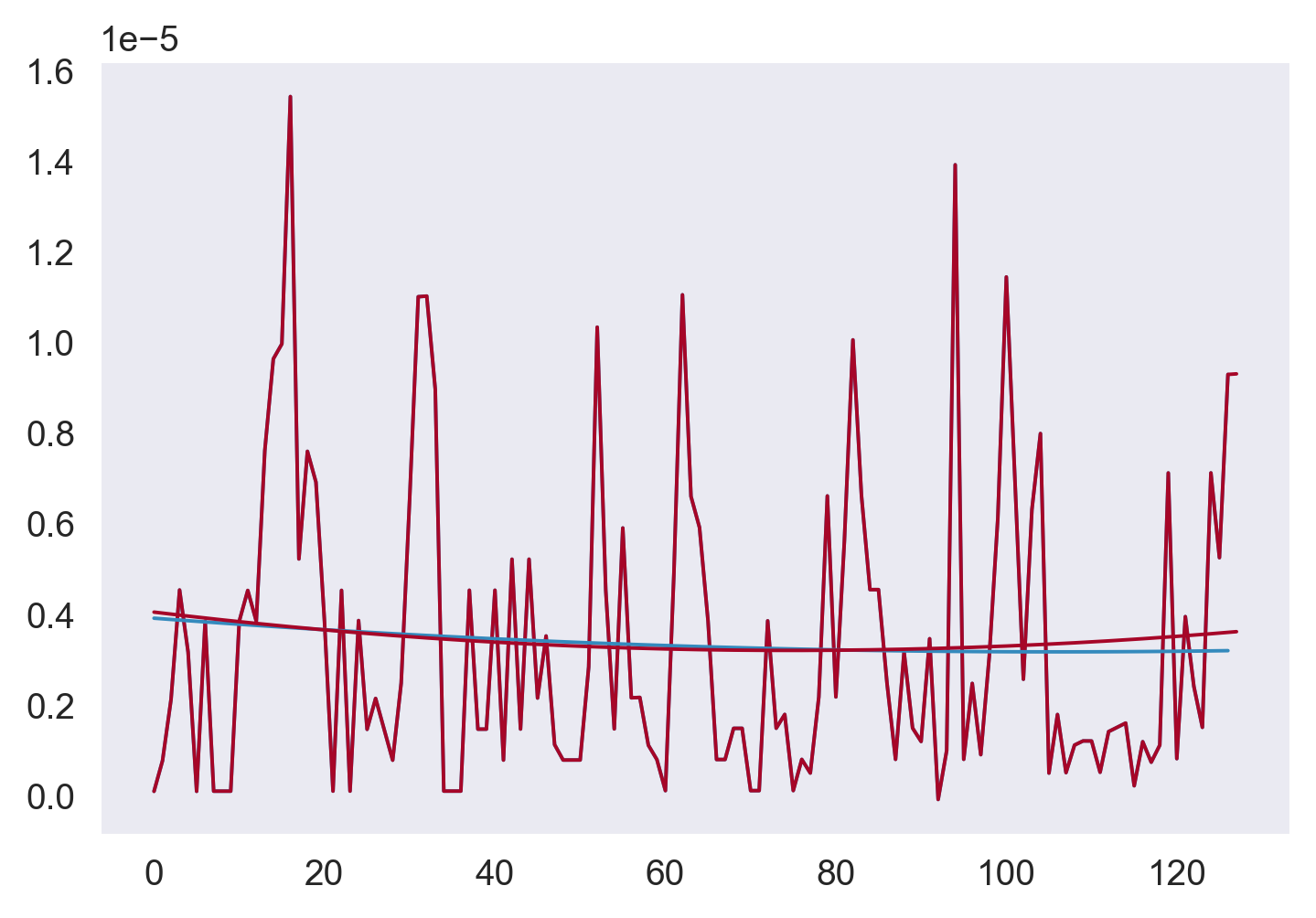
plt.figure()
plt.plot(strain[0]["N2"])
plt.plot(N2)
plt.plot(strain[0]["N2smooth"], color="C0")
plt.plot(seg.N2fit, color="C1")
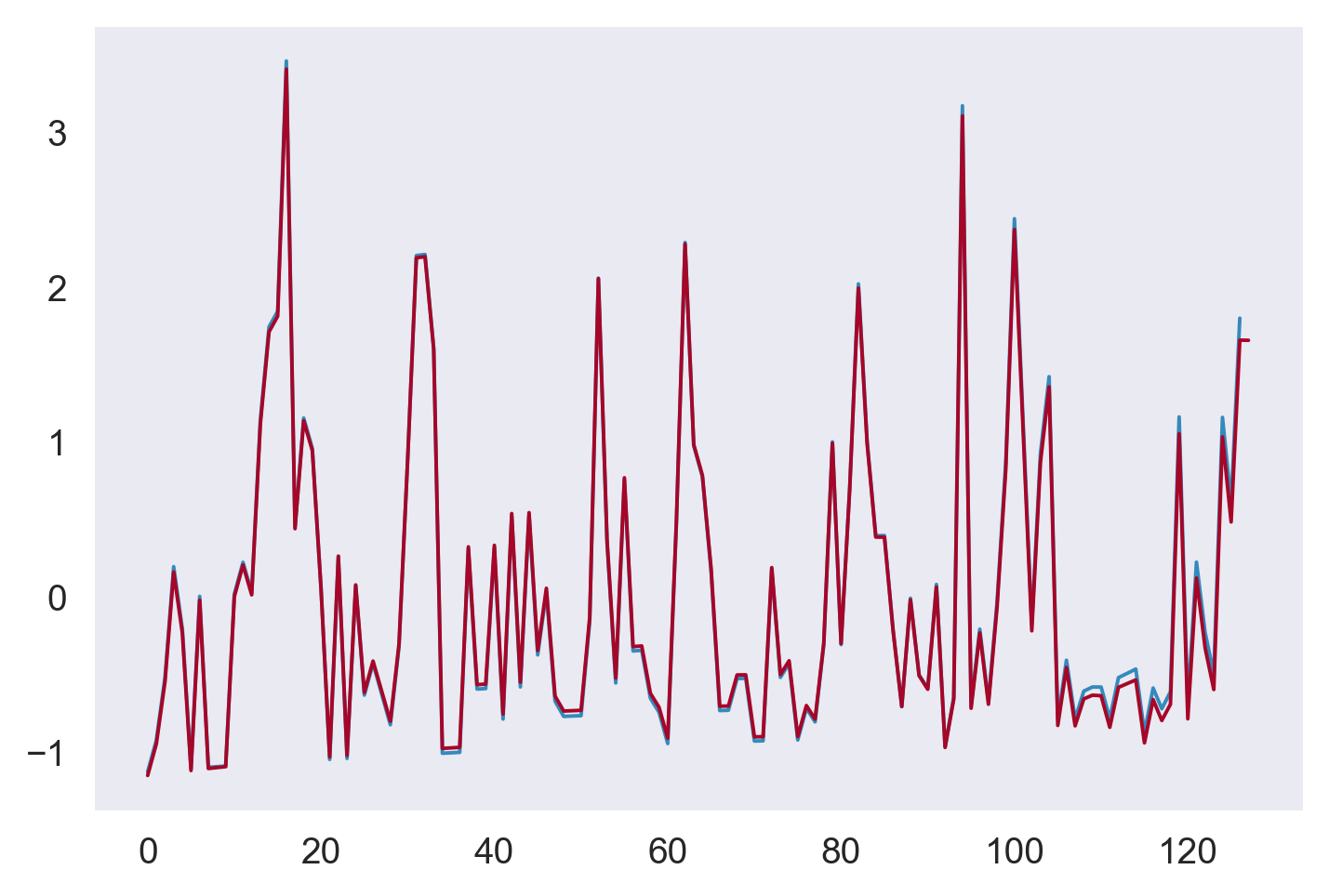
plt.figure()
plt.plot(strain[0]["strain"])
plt.plot(ξ)
0.19514013600229327 0.11266552715618153
0.1987434107341453 0.0940107853774018
[<matplotlib.lines.Line2D at 0x7f0b547b8af0>]
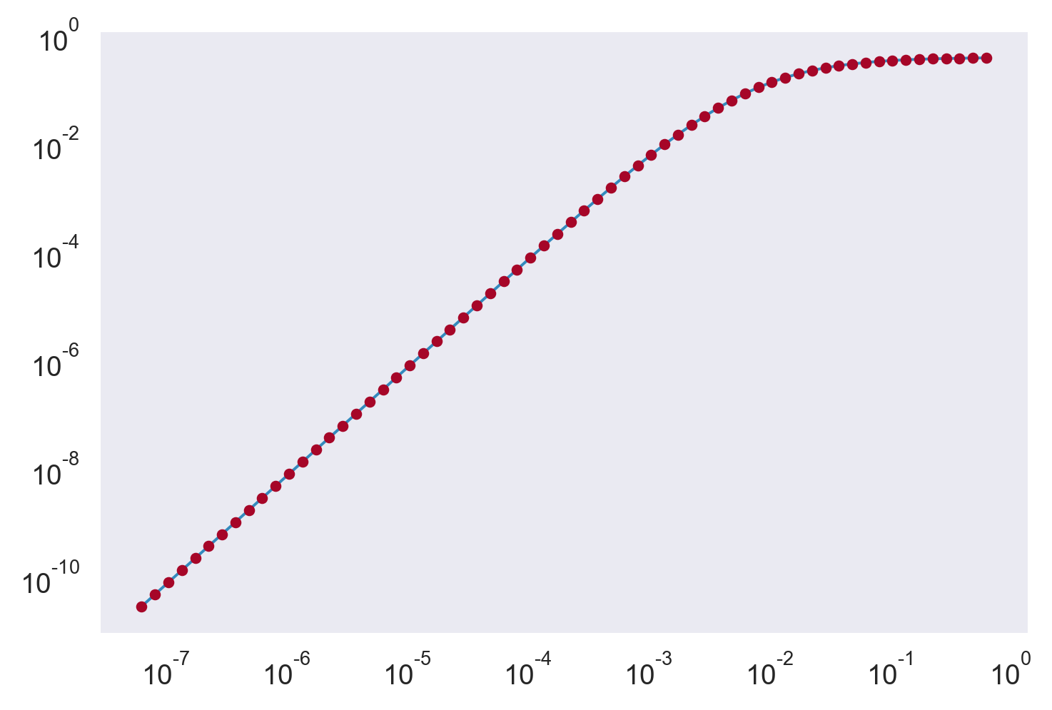
GM spectrum is right
# GM 75; Kunze et al (2017)
E0 = 6.3e-5  # nondim spectral energy level
jstar = 3  # peak mode numebr
b = 1300  # m; stratification length scale
N0 = 5.24e-3  # rad/s
K_0 = 5e-6  # m²/s for a mixing efficiency of Γ=0.2
N = N0

kz = 2 * np.pi * np.logspace(-8, -1, 64)  # np.fft.fftfreq(n=1024, d=0.1)[:64]
kzstar = (np.pi * jstar / b) * (N / N0)
ξgm = np.pi * E0 * b / 2 * jstar * kz**2 / (kz + kzstar) ** 2
plt.loglog(kz, ξgm)
print(np.trapz(ξgm, kz))

Sgm, Pgm = mixsea.shearstrain.gm_strain_variance(kz, np.arange(len(kz)), 5.24e-3)
print(Sgm)
plt.plot(kz, Pgm, ".")
0.22007432494266535
0.22007432494266535
[<matplotlib.lines.Line2D at 0x7f0b66d978e0>]
coeffs = segmented.N2.polyfit(deg=2, dim="segment")
smoothed = xr.polyval(segmented.segment, coeffs).rename(
{"polyfit_coefficients": "N2smooth"}
)
stacked = (
smoothed.transpose(..., "segment")
.assign_coords(pres=segmented.pres)
.stack({"p": ("pressure", "segment")})
)
p0, p1 = stacked.pressure.data[0], stacked.pressure.data[-1]
N2smth = (
stacked.drop("p").rename({"pres": "pressure"}).swap_dims({"p": "pressure"}).N2smooth
)
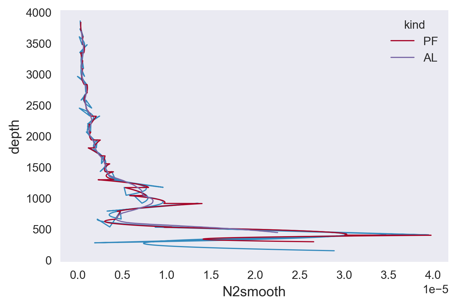
N2smth.plot(y="pressure")
mod.N2smooth.plot(y="depth", hue="kind")
[<matplotlib.lines.Line2D at 0x7f0b66b6f8b0>,
 <matplotlib.lines.Line2D at 0x7f0b66b6f8e0>]