NATRE micro vs finescale

NATRE micro vs finescale#

Here I compare the NATRE microstructure estimates with my Argo finestructure estimates. Key questions:

How well do the two agree?
- they don’t! The argo average χ seems to miss any eddy contribution; it agrees really well with the “mean stirring” estimate of Ferrari & Polzin.
If I average the microstructure to 200m bins can I recover the decomposition or not?
- TODO; skipped for now since it looks like the Argo estimate misses eddies

%load_ext watermark
%matplotlib inline

import glob

import cf_xarray as cfxr
import dask
import dcpy
import distributed
import matplotlib as mpl
import matplotlib.pyplot as plt
import numpy as np
import tqdm
from IPython.display import Image

import eddydiff as ed
import xarray as xr

xr.set_options(keep_attrs=True)

plt.rcParams["figure.dpi"] = 140
plt.rcParams["savefig.dpi"] = 200
plt.style.use("ggplot")

%watermark -iv

eddydiff   : 0.1
cf_xarray  : 0.5.3.dev29+g3660810.d20210729
numpy      : 1.21.1
dask       : 2021.7.2
tqdm       : 4.62.0
dcpy       : 0.1
xarray     : 0.17.1.dev3+g48378c4b1
matplotlib : 3.4.2
distributed: 2021.7.2

Get datasets#

There are 3

NATRE microstructure
NATRE finescale
Argo finescale

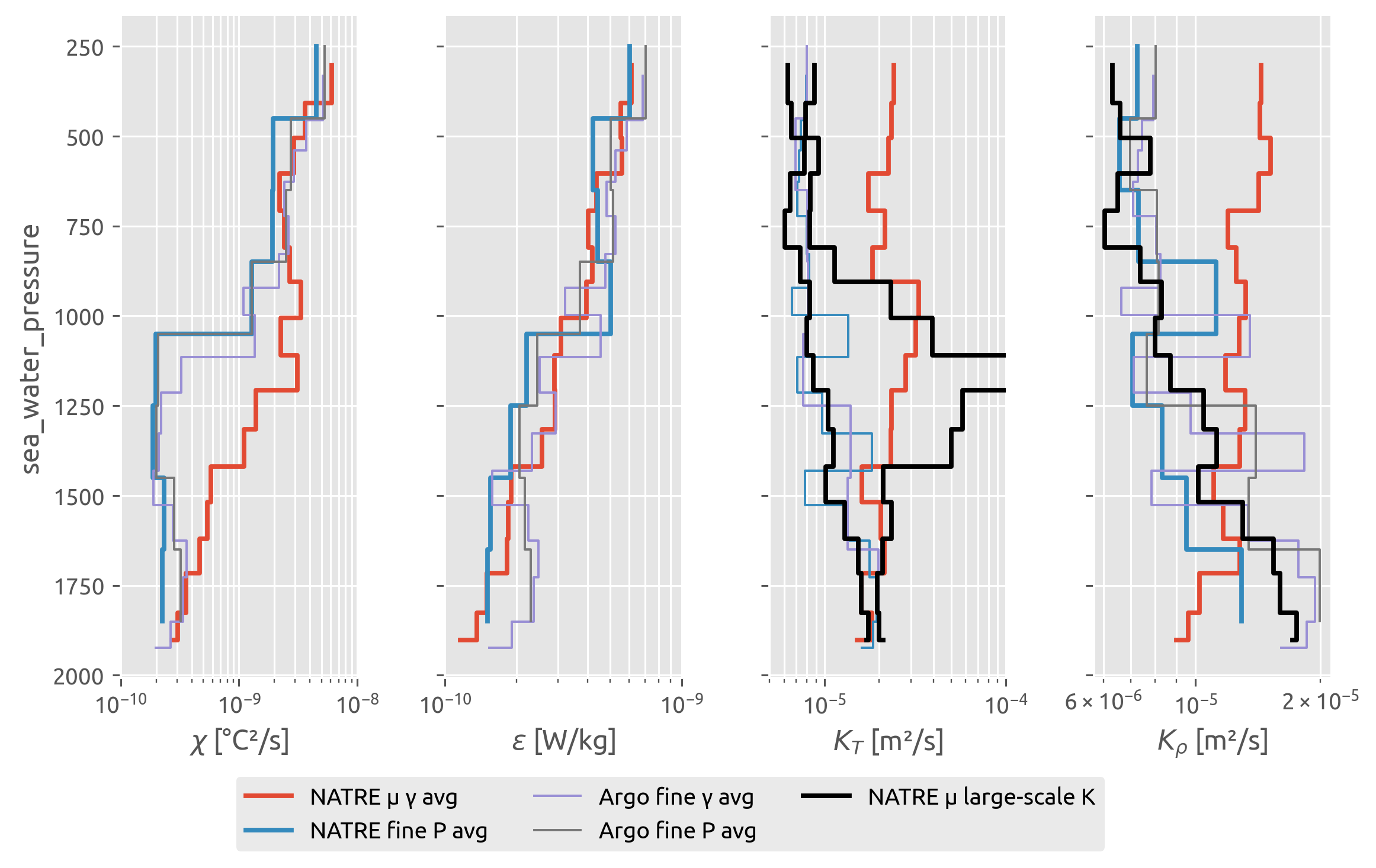
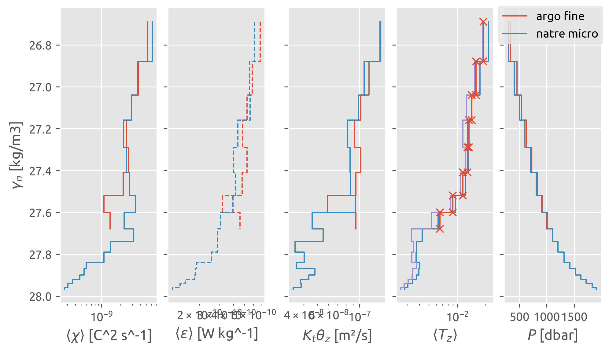
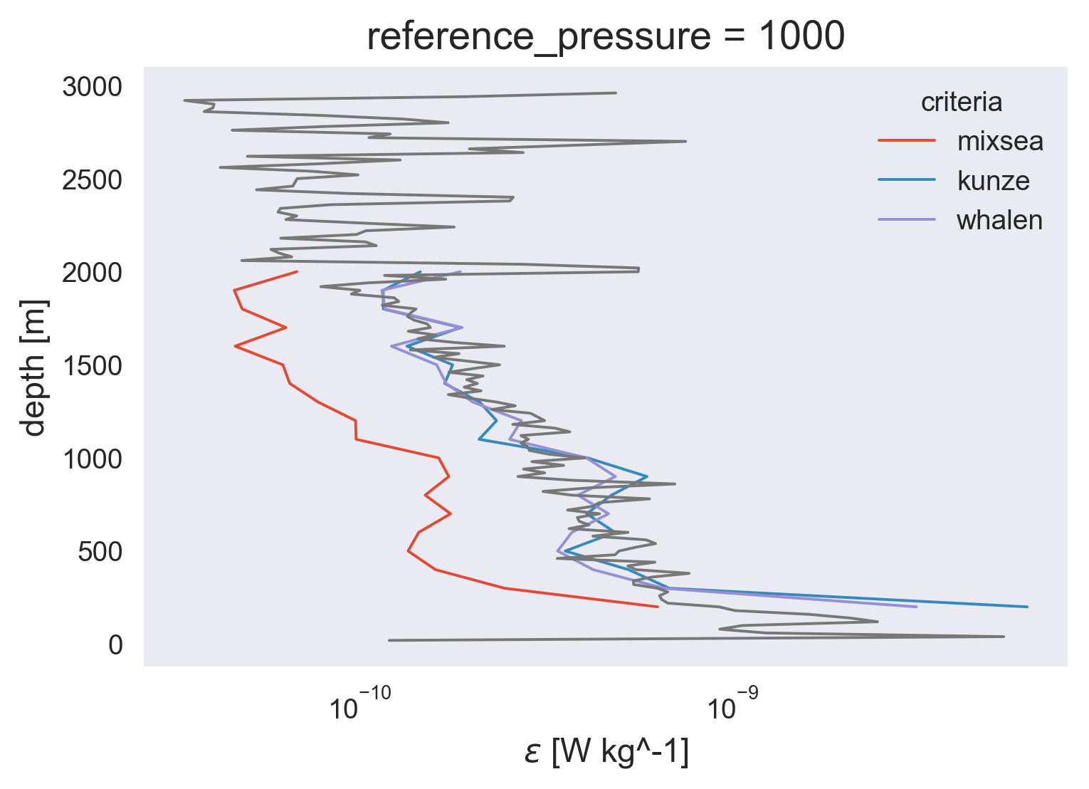
Finescale vs microscale#

The finescale \(⟨ε^{200}⟩\) estimates agree well with microscale \(⟨ε^{0.5}⟩\)
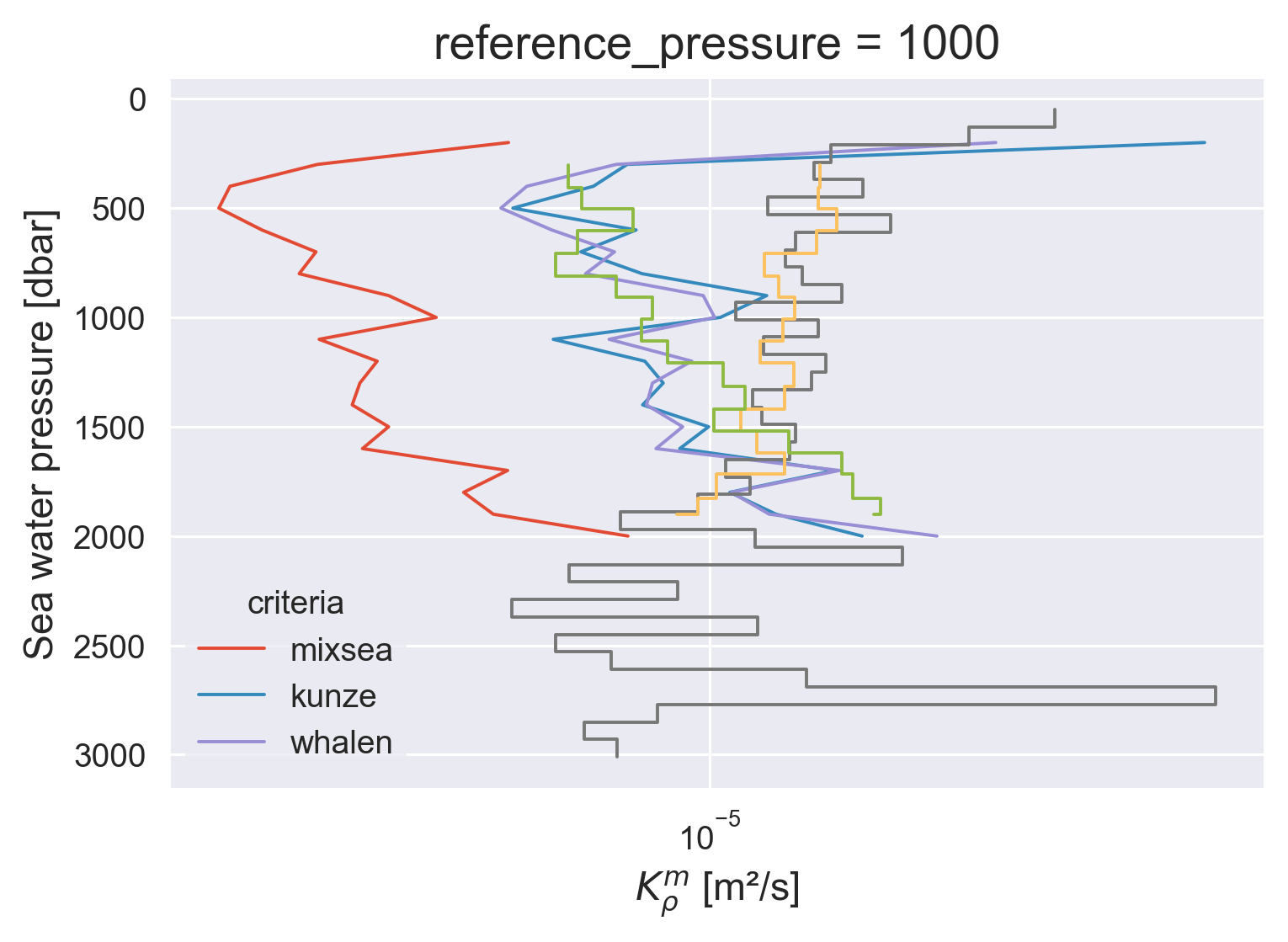
NATRE finescale \(⟨K_ρ^{200}⟩\) agrees with Argo finescale \(⟨K_ρ^{200}⟩\) which agrees with \(K_ρ^m\) \(= Γ⟨ε^{0.5}⟩/N_m^2\) i.e. a diapycnal diffusivity for the stirring of the large scale vertical gradient by the microscale. Somehow calculating a 200-m diffusivity using the finestructure \(ε^{200}\) and 200-m scale \(N²\) seems to average us out to the “large scale”
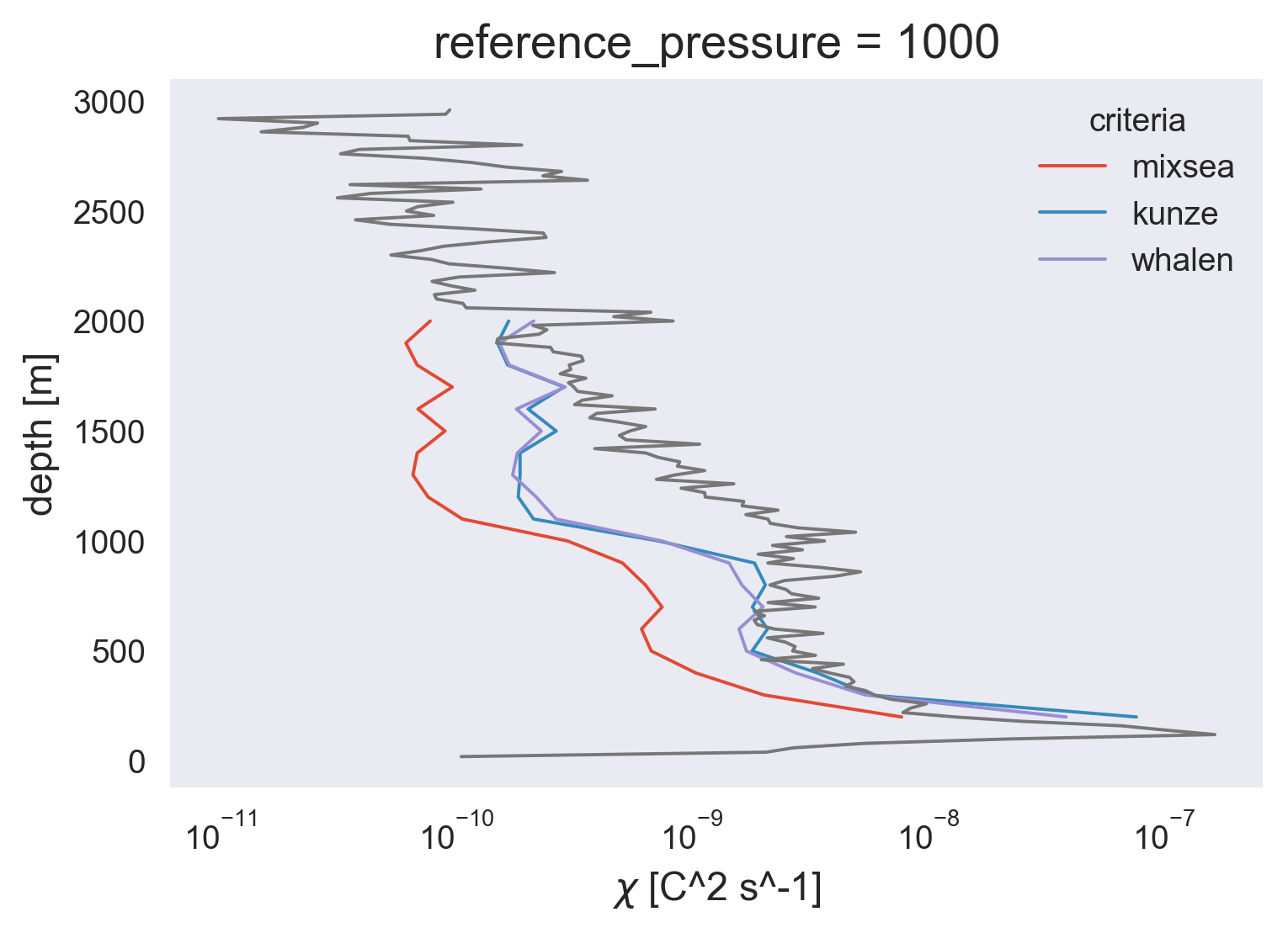
Argo finescale \(⟨χ^{200}⟩ = ⟨Γε^{200}/N\_{200}^2 ; ∂_zT\_{200}^2⟩\) seems to miss the whole eddy contribution to variance production! This is robust to averaging in γ or P, so it is not a question of the bins being too fine for the 200m mean χ estimate in each profile. I think the issue is scaling the 200-m \(ε^{200}\) with 200-m scale gradients to get \(χ^{200}\)
NATRE microscale \(⟨K_ρ⟩\) and \(⟨K_T⟩\) is quite different near the top.
The large-scale mean \(K_T^m\) is the (meaningless) diffusivity required to explain \(⟨χ⟩\) by microscale stirring on the mean vertical gradient. that’s why there’s a peak where variance is actually being generated by mesoscale stirring of the lateral gradient.

TODO:

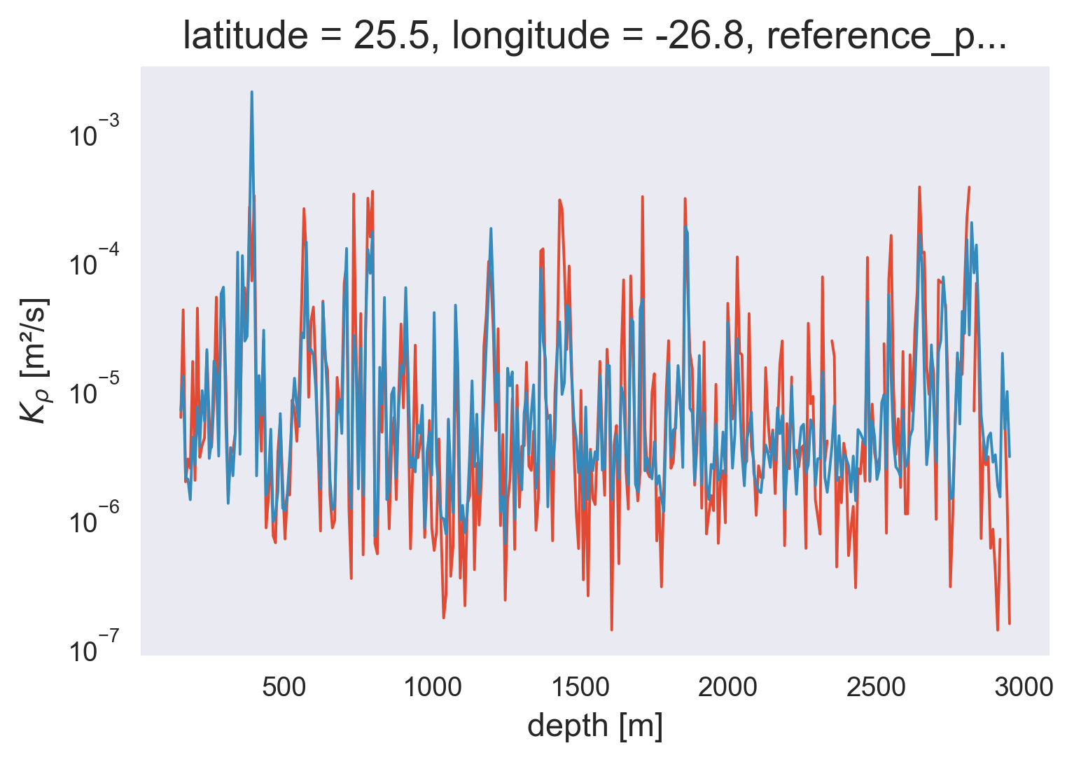
The disagreement between microscale \(⟨K_ρ⟩\) and the \(K_ρ^m\) or finescale \(K_ρ\) is the key I think. I think the 200-m averaging inherent in the finescale estimate is filtering out the mesoscale. BUT then the 200m averaged microscale \(⟨K_ρ⟩\) should also reflect this? But maybe I should calculate the 200m scale diffusivity instead of averaging the 0.5m scale diffusivity in 200m bins.
Is there any way I can estimate the microscale \(K_ρ\) that gets me back to the “large-scale” \(K_ρ^m\)
Look at individual profiles of \(χ, ε, χ^{200}, ε^{200}\); is the 200-m average taking out the eddy stirring contribution to \(T_z\)? Since they are compensated it makes sense that \(N² ≪ gαT_z^2\) at scales smaller than horizontal stirring vertical scale

_images/b3f6c6d4a9dab31ea7265765c719e7b084950cfa0c084897029737d63f6920c7.png

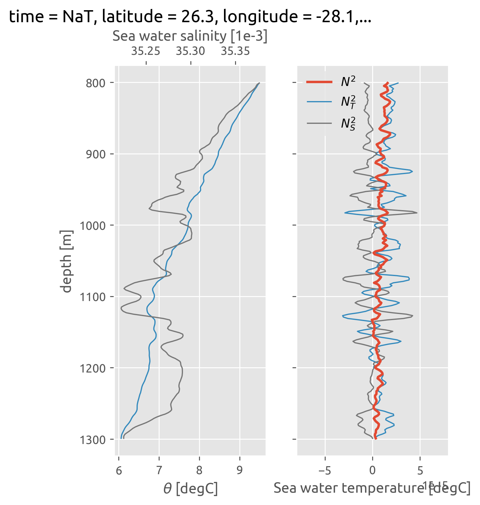
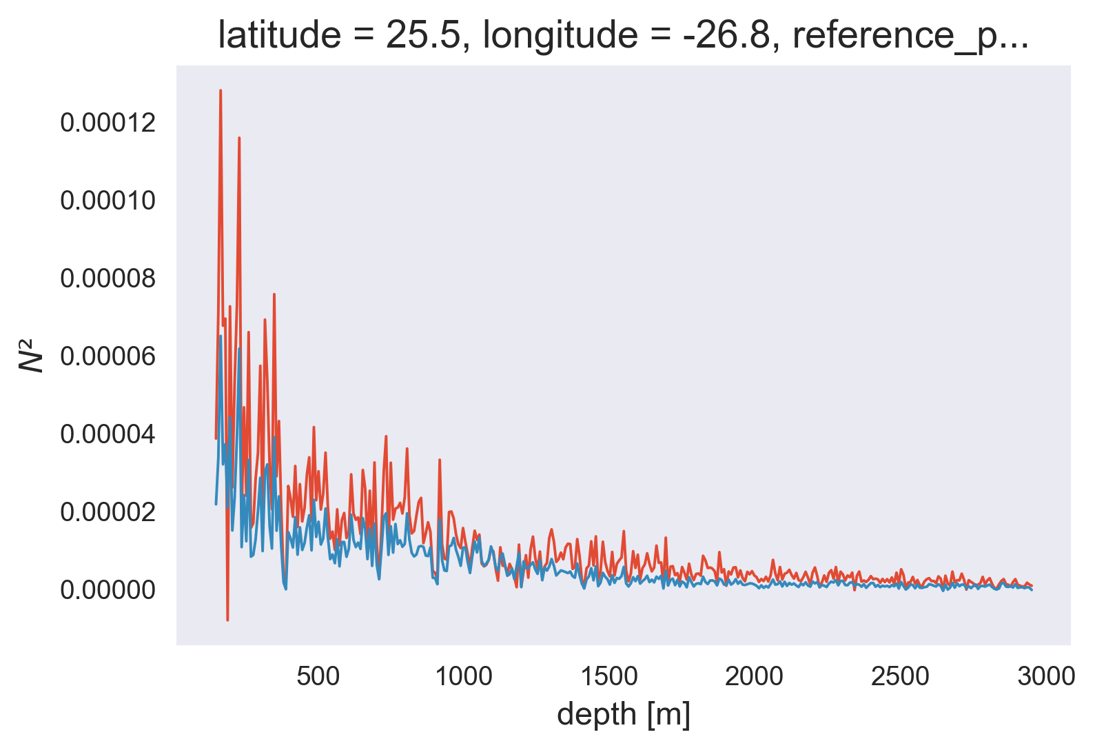
Studying N² vs \(T_z, S_z\)#

Well this is pretty clear!

There are compensated vertical gradients of \(T_z\) and \(S_z\) of ≈ 10-30m scale. So a 200-m diffusivity is acting on the much larger scale gradient \(∂_z θ_m\) not \(∂_z(θ_m + θ_e)\), the latter being the mean for the microscale diffusivity.

Another interesting thing is that \(⟨K_ρ^μ⟩ = K_ρ^m\) i.e. “large-scale” average \(K_ρ\) is the diffusivity for the “large-scale” because there is no stirring of density!

The other way to think of it is that \(K_T ≠ K_ρ\) at scales of spiciness i.e. compensated T-S variability.

profile = natre.isel(latitude=3, longitude=6).temp.interpolate_na("depth")
dcpy.ts.PlotSpectrum(profile)
dcpy.ts.PlotSpectrum(profile.rolling(depth=7, center=True).mean(), ax=plt.gca())
dcpy.ts.PlotSpectrum(profile.rolling(depth=31, center=True).mean(), ax=plt.gca())

4000000000000341
4000000000000341
4000000000000341

([<matplotlib.lines.Line2D at 0x7fc910df1910>],
 <AxesSubplot:title={'center':' Sea water temperature\n[degrees_Celsius]'}, xlabel='Wavelength/2π', ylabel='PSD'>)

%matplotlib inline
plt.rcParams["figure.dpi"] = 140

profile = (
    natre.isel(latitude=3, longitude=6)
    .rolling(depth=21, center=True, min_periods=1)
    .mean()
    .coarsen(depth=5, boundary="trim")
    .mean()
    .sel(depth=slice(800, 1300))
)

profile["NT2"] = (
    -9.81
    * dcpy.eos.alpha(profile.salt, profile.temp, profile.pres)
    * profile.theta.interpolate_na("depth").differentiate("depth")
)
profile["NS2"] = (
    9.81
    * dcpy.eos.beta(profile.salt, profile.temp, profile.pres)
    * profile.salt.interpolate_na("depth").differentiate("depth")
)

f, ax = plt.subplots(1, 2, sharey=True)

profile.theta.cf.plot(ax=ax[0], color="C1")

axS = ax[0].twiny()
axS.grid(False)
profile.salt.cf.plot(color="C3", ax=axS)

# ax2 = ax[0].twiny()
# profile.gamma_n.cf.plot(color="k", ax=ax2)
# ax2.grid(False)

profile.N2.cf.plot(lw=2, zorder=5, ax=ax[1])
profile.NT2.cf.plot(ax=ax[1])
profile.NS2.cf.plot(color="C3", ax=ax[1])
ax[1].set_xlim([-8e-5, 8e-5])
ax[1].legend(["$N^2$", "$N_T^2$", "$N_S^2$"])

dcpy.plots.clean_axes(ax)
[aa.set_title("") for aa in ax]

f.set_size_inches((5, 6))

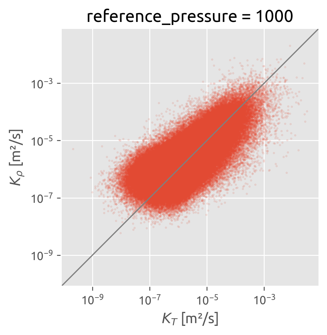
_images/78da85eeaecbfd567cef3e0d23d58ea6105c8f7bc8b217db86d49ee619e85fa6.png

Studying \(K_T\) vs \(K_ρ\)#

I’m wondering if the \(K_T = K_ρ\) assumption really breaks down at the 200-m scale?

calculate \(K_T, K_ρ\) from the microstructure data at various averaging scales.

natre.plot.scatter(x="Kt", y="Krho", s=2, alpha=0.1)
plt.gca().set_xscale("log")
plt.gca().set_yscale("log")
dcpy.plots.line45()

_images/5ba2701e1eae3b444f87694c3413977e6c3eba05c2957a32a6d3c448e6158d2f.png

Old stuff#

def decode_bounds_to_intervals(dataset, bounds_dim="bounds"):

    dataset = dataset.copy(deep=True)
    all_bounds = dataset.cf.bounds
    for name in set(dataset.variables) & set(all_bounds):
        bounds_name = all_bounds[name][0]
        vertices = cfxr.bounds_to_vertices(dataset[bounds_name], bounds_dim)
        intervals = ed.intervals_from_vertex(vertices)
        dataset[name] = dataset[name].copy(data=intervals)
        del dataset[name].attrs["bounds"]
        dataset = dataset.drop(bounds_name)
    return dataset


micro = decode_bounds_to_intervals(micro)

argo_fine.npts.plot()

[<matplotlib.lines.Line2D at 0x7ff00197a6a0>]

_images/adcda13d528b368f79d5d5226e43b099f2a05ef30b53a1805d01df063ff37d3e.png

f, ax = plt.subplots(1, 5, sharey=True, constrained_layout=True)
kwargs = dict(y="neutral_density", xscale="log")

argo_fine.gamma_n_bins.attrs["standard_name"] = "neutral_density"
masked_argo_fine = argo_fine.where(argo_fine.npts > 300)
for var in argo_fine.variables:
    masked_argo_fine[var].attrs = argo_fine[var].attrs

masked_argo_fine.χ.cf.plot.step(ax=ax[0], **kwargs)
micro.chi.cf.plot.step(ax=ax[0], **kwargs)

masked_argo_fine.ε.cf.plot.step(ax=ax[1], color="C0", ls="--", **kwargs)
micro.eps.cf.plot.step(ax=ax[1], color="C1", ls="--", **kwargs)

masked_argo_fine.KtTz.cf.plot.step(ax=ax[2], **kwargs)
micro.KtTz.cf.plot.step(ax=ax[2], **kwargs)
# micro.KrhoTz.cf.plot.step(ax=ax[2], **kwargs)

masked_argo_fine.Tzmean.cf.plot.step(ax=ax[3], **kwargs)
micro.Tz.cf.plot.step(ax=ax[3], **kwargs)
micro.dTdz_m.cf.plot.step(ax=ax[3], **kwargs)
masked_argo_fine.mean_dTdz_seg.cf.plot.step(ax=ax[3], color="C0", marker="x", **kwargs)

masked_argo_fine.pressure.cf.plot.step(ax=ax[4], y="neutral_density")
micro.pres.cf.plot.step(ax=ax[4], y="neutral_density")

ax[-1].set_xlabel("$P$ [dbar]")
f.legend(["argo fine", "natre micro"])
dcpy.plots.clean_axes(ax)
[aa.set_title("") for aa in ax]
f.set_size_inches((7, 4))

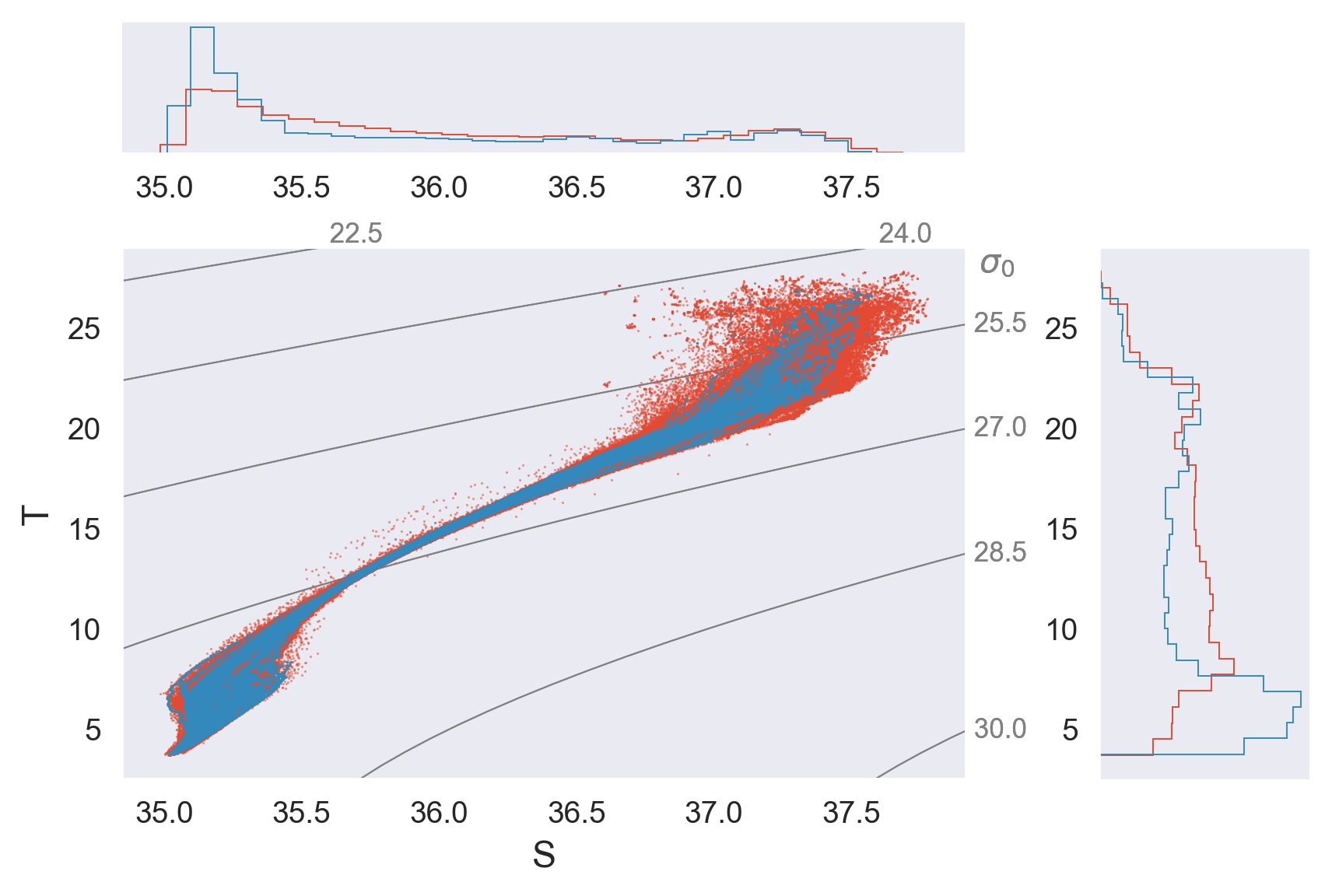
_images/10d289cca05a927e81be506045c50af9bbc30ee4103a9e859d6c3bab2c4d8612.png

T-S#

Hmm.. the T-S diagram for Argo profiles with which we can calculate finescale estimates should tell us if it samples any eddy stirring at all.

argo_fine_full_profiles = xr.load_dataset("argo_profiles_used_for_finestructure.nc")

mask = argo_fine_full_profiles.fine_deepest_bin > 1200

kwargs = dict(hexbin=False, size=0.1)

_, ax = dcpy.oceans.TSplot(
    argo_fine_full_profiles.PSAL,
    argo_fine_full_profiles.THETA,
    **kwargs,
)
dcpy.oceans.TSplot(
    argo_fine_full_profiles.where(mask, drop=True).PSAL,
    argo_fine_full_profiles.where(mask, drop=True).THETA,
    **kwargs,
    ax=ax,
);

_images/3a29e23fd7827c81aefe9d77739b02aa7451699e21bf3b8389b25446d78c3db0.png

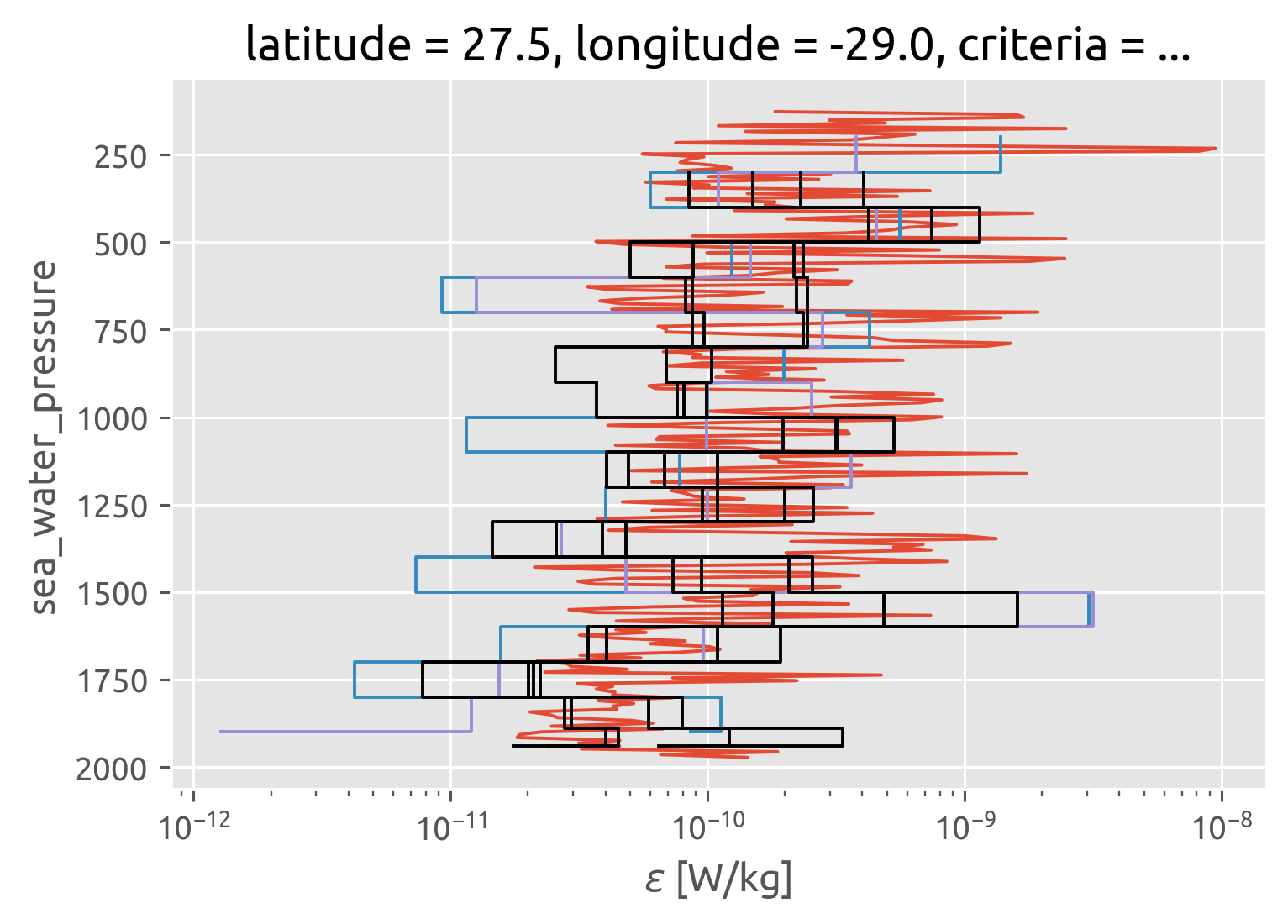
Finescale estimate with NATRE data#

def fix_profile(profile):

    fixed = (
        profile.unstack()
        .squeeze()
        .cf.guess_coord_axis()
        .cf.dropna("Z", how="any")
        .set_coords("pres")
        .drop("depth")
        .swap_dims({"depth": "pres"})
    )

    assert fixed.temp.isnull().sum() == 0
    return fixed


stacked = (
    natre.load()
    .reset_coords("pres")
    .cf.interpolate_na("Z")
    .stack({"latlon": ["longitude", "latitude"]})
)

results = [
    dask.delayed(dcpy.finestructure.process_profile)(
        fix_profile(stacked.isel(latlon=[idx]))
    )
    for idx in range(1, stacked.sizes["latlon"])
]

profile = fix_profile(stacked.isel(latlon=[40]))
ms = dcpy.finestructure.do_mixsea_shearstrain(profile, dz_segment=200)
dc = dcpy.finestructure.process_profile(profile, dz_segment=200, criteria=None)

profile.eps.coarsen(pres=20, boundary="trim").mean().plot(y="pres")
ms.eps.isel(kind=0).plot.step(y="depth_bin", xscale="log", yincrease=False)
ms.eps.isel(kind=1).plot.step(y="depth_bin", xscale="log", yincrease=False)
for crit in dc.criteria:
    dc.sel(criteria=crit).ε.cf.plot.step(color="k")

_images/34505b5cee4caba0edabd22731bf9ff304f3c5bd7f80b1a95a8e601b3e62e62f.png

from dask.distributed import Client

client = Client("tcp://127.0.0.1:41667")
client

Client

Client-a53a850d-e9a0-11eb-8526-0028f8270ea7

Connection method: Direct
Dashboard: http://127.0.0.1:8787/status

Scheduler Info

Scheduler

Scheduler-d6f7fb0f-8f7b-4ee3-8176-31ebb7885697

Comm: tcp://127.0.0.1:41667	Workers: 4
Dashboard: http://127.0.0.1:8787/status	Total threads: 8
Started: 1 minute ago	Total memory: 31.10 GiB

Workers

Worker: 0

Comm: tcp://127.0.0.1:38589	Total threads: 2
Dashboard: http://127.0.0.1:38143/status	Memory: 7.77 GiB
Nanny: tcp://127.0.0.1:45089
Local directory: /tmp/dask-worker-space/worker-j3tr7azt
Tasks executing: 0	Tasks in memory: 0
Tasks ready: 0	Tasks in flight: 0
CPU usage: 2.0%	Last seen: Just now
Memory usage: 307.97 MiB	Spilled bytes: 0 B
Read bytes: 84.62 kiB	Write bytes: 5.47 MiB

Worker: 1

Comm: tcp://127.0.0.1:34279	Total threads: 2
Dashboard: http://127.0.0.1:36725/status	Memory: 7.77 GiB
Nanny: tcp://127.0.0.1:45517
Local directory: /tmp/dask-worker-space/worker-3ble6b2n
Tasks executing: 0	Tasks in memory: 0
Tasks ready: 0	Tasks in flight: 0
CPU usage: 2.0%	Last seen: Just now
Memory usage: 305.44 MiB	Spilled bytes: 0 B
Read bytes: 102.43 kiB	Write bytes: 12.61 MiB

Worker: 2

Comm: tcp://127.0.0.1:36211	Total threads: 2
Dashboard: http://127.0.0.1:45765/status	Memory: 7.77 GiB
Nanny: tcp://127.0.0.1:33209
Local directory: /tmp/dask-worker-space/worker-oa6g1apu
Tasks executing: 0	Tasks in memory: 0
Tasks ready: 0	Tasks in flight: 0
CPU usage: 2.0%	Last seen: Just now
Memory usage: 304.01 MiB	Spilled bytes: 0 B
Read bytes: 86.19 kiB	Write bytes: 5.47 MiB

Worker: 3

Comm: tcp://127.0.0.1:43585	Total threads: 2
Dashboard: http://127.0.0.1:45443/status	Memory: 7.77 GiB
Nanny: tcp://127.0.0.1:37171
Local directory: /tmp/dask-worker-space/worker-hnwyf6y6
Tasks executing: 0	Tasks in memory: 0
Tasks ready: 0	Tasks in flight: 0
CPU usage: 4.0%	Last seen: Just now
Memory usage: 306.35 MiB	Spilled bytes: 0 B
Read bytes: 62.84 kiB	Write bytes: 8.10 MiB

computed = dask.compute(results, scheduler="threads")

/home/deepak/work/python/dcpy/dcpy/finestructure.py:311: RuntimeWarning: invalid value encountered in true_divide
  scale = (ξvar / ξgmvar) ** 2 * h_Rω * L_Nf
/home/deepak/work/python/dcpy/dcpy/finestructure.py:311: RuntimeWarning: invalid value encountered in true_divide
  scale = (ξvar / ξgmvar) ** 2 * h_Rω * L_Nf

def fix_result(profile):
    return (
        profile.rename_dims({"pressure": "pressure_"})
        .reset_coords()
        .set_coords(["latitude", "longitude"])
        .expand_dims(["latitude", "longitude"])
        .assign_coords({"pressure_": np.arange(profile.sizes["pressure"])})
    )


combined = xr.combine_by_coords([fix_result(ds) for ds in computed[0]])
combined = combined.cf.guess_coord_axis()

combined.to_netcdf("../datasets/natre-finescale.nc")

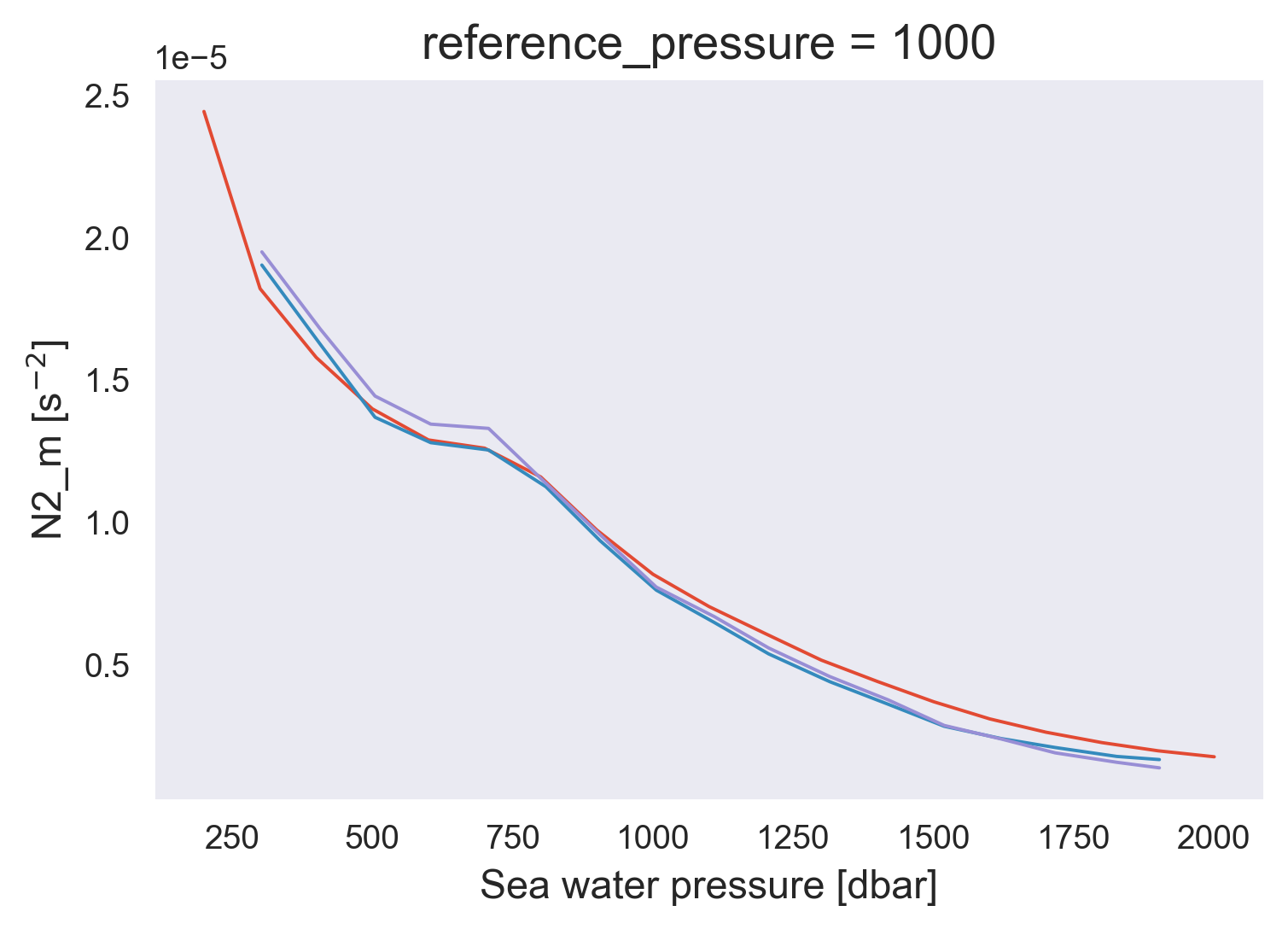
avg = combined.groupby_bins("pressure", np.arange(150, 2060, 100)).mean()

avg.N2mean.plot()
micro.N2.plot(x="pres")
micro.N2_m.plot(x="pres")

[<matplotlib.lines.Line2D at 0x7fefa3e34760>]

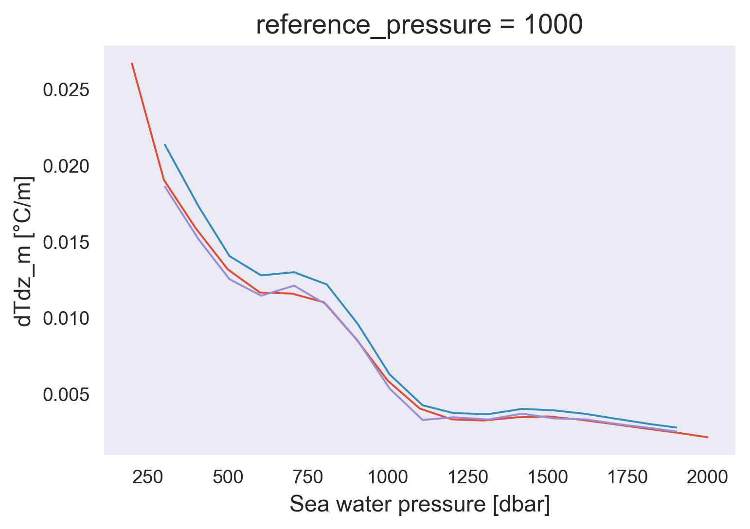
_images/2cf65900c13d0246b2eb27bae8c487cdbb092de043acc53ef3f1be66f252dfc8.png

avg.Tzmean.plot()
micro.Tz.plot(x="pres")
micro.dTdz_m.plot(x="pres")

[<matplotlib.lines.Line2D at 0x7feff10f9400>]

_images/ff5ce46217218d5e4e8d19a565eaf8d7c4085f0ec8c153906bf6407c7ede9bba.png

avg.ε.plot(y="pressure_bins", hue="criteria", xscale="log")
natre.eps.mean(["latitude", "longitude"]).coarsen(
    depth=50, boundary="trim"
).mean().plot(y="depth")

[<matplotlib.lines.Line2D at 0x7fefdd4f9eb0>]

_images/ae13c3604e4a92b9005fe7feea88edd4d8d20d04f22c8a3499dbadc49f138278.png

(avg.Kρ).plot(y="pressure_bins", hue="criteria", xscale="log")
natre.Krho.coarsen(depth=200, boundary="trim").mean().mean(
    ["latitude", "longitude"]
).plot.step(y="depth")
micro.Krho.plot.step(y="pres")
micro.Krho_m.plot.step(y="pres", yincrease=False)
plt.gca().grid(True)

_images/0f6efce69e9d28ea0eb1a9cd425236077e0919b6177b31ba3b138cc9680763b2.png

(avg.χ).plot(y="pressure_bins", hue="criteria", xscale="log")
natre.chi.mean(["latitude", "longitude"]).coarsen(
    depth=50, boundary="trim"
).mean().plot(y="depth")

[<matplotlib.lines.Line2D at 0x7fefe462fc10>]

_images/cb4e7efdf4d2a9d01792ae1ef197b19f951f75e9fb6747dc118b90bdbe95ddf8.png

(9.81 * 1.7e-4 * profile.Tz).plot()
profile.N2.plot()

[<matplotlib.lines.Line2D at 0x7fefdc273d30>]

_images/0a28e43d98befc2ed1a78a358f45b1c58231a5e17c5cc901bb4cbeb0b29b2a72.png

profile = natre.isel(latitude=5, longitude=9).coarsen(depth=20, boundary="trim").mean()

profile.Kt.plot()
profile.Krho.plot(yscale="log")

[<matplotlib.lines.Line2D at 0x7fefddf66670>]

_images/b36df46760fa01e459374633ccc29ab55d492f6904e2b5de98eef9822ddc1b79.png