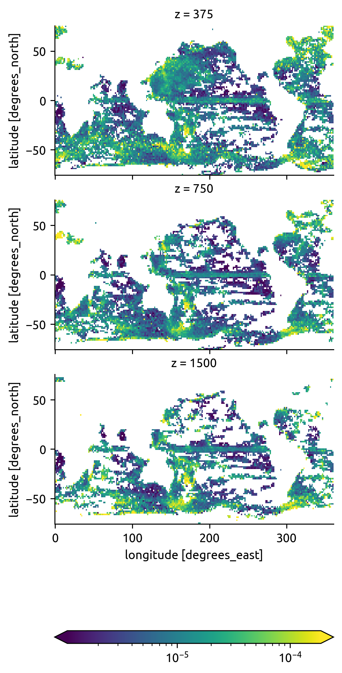
Existing finestructure estimates

1. Whalen’s estimates are in pretty large bins 250-500m; 500m-1000m; 1000m-2000m; and there’s lot of data missing in the NATRE region

import cf_xarray
import dcpy
import gsw
import matplotlib as mpl
import mixsea
import pandas as pd
import scipy
import scipy.integrate
import seawater as sw
from scipy import signal
from scipy.io import loadmat

import xarray as xr

mpl.rcParams["figure.dpi"] = 140
dirname = "/home/deepak/datasets/finestructure/"

Whalen

Sneakily taken from acknowledgments of Trossman et al (2020)

K = []
for z, name in zip((375, 750, 1500), ["250to500m", "500to1000m", "1000to2000m"]):
    mat = loadmat(f"{dirname}/whalen/av_world_K_{name}_3_1p5deg_2015.mat")
    K.append(
        xr.DataArray(
            mat["c"],
            dims=("lat", "lon"),
            coords={"lat": mat["y"].squeeze(), "lon": mat["x"].squeeze(), "z": z},
        )
    )

K = xr.concat(K, dim="z").cf.guess_coord_axis()
K.z.attrs["units"] = "m"
K.to_netcdf(f"{dirname}/whalen2015.nc")
K

<xarray.DataArray (z: 3, lat: 101, lon: 241)>
array([[[1.14926924e-03, 1.87404820e-03,            nan, ...,
         1.73270825e-03, 1.19684959e-04, 4.04780348e-04],
        [4.61545906e-05, 3.77968734e-05, 2.20720928e-03, ...,
                    nan, 8.46056775e-05, 2.20150150e-05],
        [           nan, 3.64251173e-05, 2.34609923e-05, ...,
         1.72037751e-05, 1.85861537e-04, 9.51779934e-06],
        ...,
        [           nan,            nan,            nan, ...,
                    nan,            nan,            nan],
        [           nan,            nan,            nan, ...,
                    nan,            nan,            nan],
        [           nan,            nan,            nan, ...,
                    nan,            nan,            nan]],

       [[6.74521750e-04, 1.62954533e-04,            nan, ...,
         1.75821579e-04, 9.47196336e-06, 1.19420112e-05],
        [           nan,            nan, 1.19879684e-04, ...,
                    nan, 2.72826324e-05,            nan],
        [1.36392184e-05, 4.14167208e-05, 4.26732736e-05, ...,
                    nan, 1.34894389e-04, 1.08020983e-05],
...
        [           nan,            nan,            nan, ...,
                    nan,            nan,            nan],
        [           nan,            nan,            nan, ...,
                    nan,            nan,            nan],
        [           nan,            nan,            nan, ...,
                    nan,            nan,            nan]],

       [[           nan,            nan,            nan, ...,
                    nan,            nan,            nan],
        [           nan,            nan,            nan, ...,
                    nan,            nan,            nan],
        [           nan, 5.37029196e-06, 2.99769652e-05, ...,
                    nan,            nan,            nan],
        ...,
        [           nan,            nan,            nan, ...,
                    nan,            nan,            nan],
        [           nan,            nan,            nan, ...,
                    nan,            nan,            nan],
        [           nan,            nan,            nan, ...,
                    nan,            nan,            nan]]])
Coordinates:
  * lat      (lat) float64 75.0 73.5 72.0 70.5 69.0 ... -70.5 -72.0 -73.5 -75.0
  * lon      (lon) float64 0.0 1.5 3.0 4.5 6.0 ... 354.0 355.5 357.0 358.5 360.0
  * z        (z) int64 375 750 1500

K.plot(
    row="z",
    norm=mpl.colors.LogNorm(),
    robust=True,
    cbar_kwargs={"orientation": "horizontal"},
)

<xarray.plot.facetgrid.FacetGrid at 0x7fbbc06bbb50>

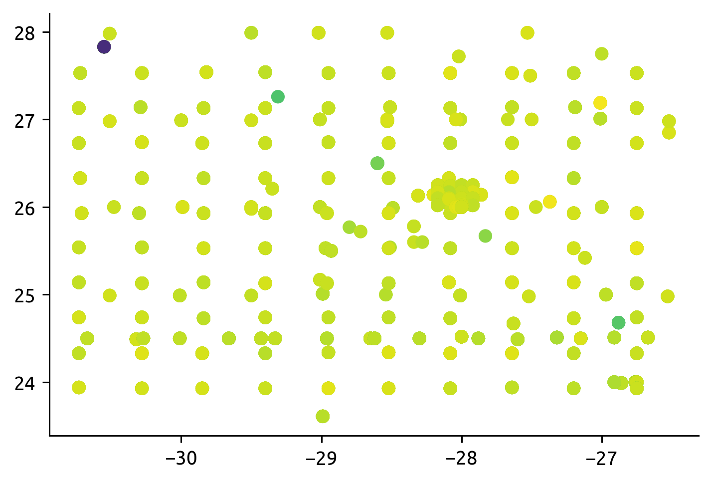
Kunze

The remaining lines list

• hydrographic section name,

• the drop number,

• latitude,

• longitude,

• bounding depths z_i and z_f,

• bounding neutral densities,

• buoyancy frequency squared N^2,

• dissipation rate (W/kg)

• diapycnal diffusivity K (m^2/s).

kunze = dcpy.oceans.read_kunze_2017_finestructure()

natre_fs = kunze.query(
    "longitude > -31 & longitude < -26.5 & latitude > 23.5 & latitude < 28"
)

import matplotlib.pyplot as plt
import numpy as np

plt.scatter(natre_fs["longitude"], natre_fs["latitude"], c=np.log10(natre_fs["ε"]))

<matplotlib.collections.PathCollection at 0x7fbb0f40dc10>

factorized = pd.cut(
    kunze.γ_mean,
    bins=[
        26.692,
        26.876,
        27.039,
        27.163,
        27.288,
        27.406,
        27.516,
        27.605,
        27.683,
        27.742,
        27.794,
        27.835,
        27.872,
        27.898,
        27.921,
        27.94,
        27.958,
    ],
)
binned = kunze.groupby(factorized).mean()
binned.index = binned["γ_mean"]
binned = binned.to_xarray().set_coords("z_mean")
binned

<xarray.Dataset>
Dimensions:    (γ_mean: 16)
Coordinates:
  * γ_mean     (γ_mean) float64 26.79 26.96 27.1 27.23 ... 27.91 27.93 27.95
    z_mean     (γ_mean) float64 -399.5 -438.7 -487.1 ... -1.569e+03 -1.728e+03
Data variables:
    drop       (γ_mean) float64 57.68 58.92 58.71 55.09 ... 50.61 51.6 51.83
    latitude   (γ_mean) float64 3.025 4.287 6.493 11.97 ... 28.51 28.81 27.91
    longitude  (γ_mean) float64 -35.37 -31.95 -31.62 ... -33.96 -33.79 -34.44
    z_i        (γ_mean) float64 -271.9 -311.8 -361.2 ... -1.443e+03 -1.602e+03
    z_f        (γ_mean) float64 -527.1 -565.6 -613.0 ... -1.696e+03 -1.854e+03
    γ_i        (γ_mean) float64 26.55 26.75 26.94 27.11 ... 27.89 27.91 27.93
    γ_f        (γ_mean) float64 27.04 27.18 27.27 27.35 ... 27.93 27.95 27.97
    N2         (γ_mean) float64 1.579e-05 1.352e-05 ... 1.104e-06 9.568e-07
    ε          (γ_mean) float64 2.353e-09 1.943e-09 ... 2.236e-10 1.829e-10
    K          (γ_mean) float64 3.272e-05 3.275e-05 ... 5.24e-05 4.898e-05

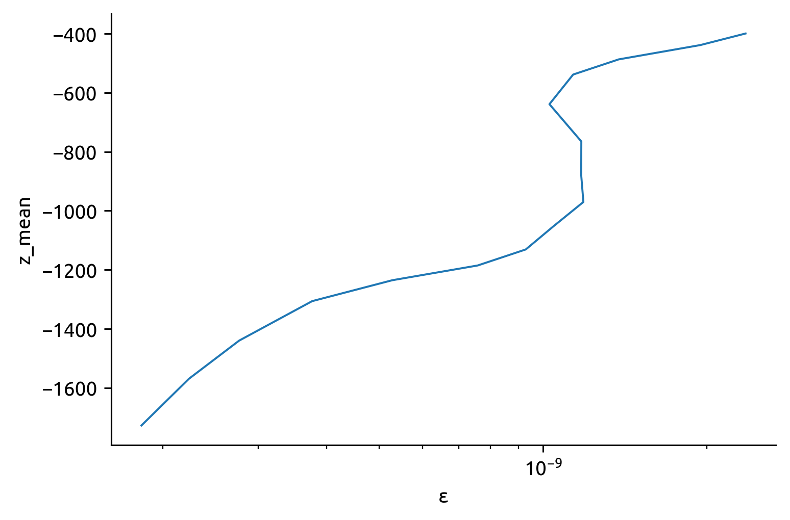
This looks encouraging; ε is elevated in the same depth range where χ is elevated

binned.ε.plot(y="z_mean", xscale="log")

[<matplotlib.lines.Line2D at 0x7fbb4a581790>]

kunze.groupby("cruise").count()

	drop	latitude	longitude	z_i	z_f	γ_i	γ_f	N2	ε	K	z_mean	γ_mean
cruise
06AQ19860627	189	189	128	189	189	189	189	189	189	189	189	189
06AQ19931212	502	502	446	502	502	502	502	502	502	502	502	502
317519930704	2117	2117	2117	2117	2117	2117	2117	2117	2117	2117	2117	2117
32OC20080510	270	270	270	270	270	270	270	270	270	270	270	270
64PE20050907	1163	1163	1163	1163	1163	1163	1163	1163	1163	1163	1163	1163
...	...	...	...	...	...	...	...	...	...	...	...	...
ar24_b	1955	1955	1955	1955	1955	1955	1955	1955	1955	1955	1955	1955
ar25_h	496	496	496	496	496	496	496	496	496	496	496	496
atas1	85	85	85	85	85	85	85	85	85	85	85	85
atas2	129	129	129	129	129	129	129	129	129	129	129	129
atas3	196	196	196	196	196	196	196	196	196	196	196	196

135 rows × 12 columns