TAO (0, 140) χpod#
TODO#
1023.5 surface does not exist south of 2N? Something is weird. More generally how do I deal with ECCO bias? Or I need to choose bins based on outcrops I guess
Argo spline fits are a little steep
Estimate gradients at latitude=0, exactly
Understand regrid_conservative: Am I providign bin edges or bin centers.
Then do the right thing to get derivative.
Think about EUC max
%load_ext watermark

import cf_xarray
import dcpy
import distributed
import hvplot.xarray
import matplotlib as mpl
import matplotlib.pyplot as plt
import numpy as np
import pandas as pd
import pump
import xgcm

import eddydiff as ed
import xarray as xr

xr.set_options(keep_attrs=True)

%watermark -iv
plt.rcParams["figure.dpi"] = 180
plt.rcParams["savefig.dpi"] = 200

client = distributed.Client()
client
xgcm       : 0.5.1
pump       : 0.1
hvplot     : 0.7.1
distributed: 2021.3.0
dcpy       : 0.1
pandas     : 1.2.3
cf_xarray  : 0.4.1.dev21+gab9dc66
xarray     : 0.17.1.dev3+g48378c4b1
matplotlib : 3.3.4
eddydiff   : 0.1
numpy      : 1.20.1
Client
|
Cluster
|
Read χpod , TAO data#
chi = (
    xr.open_dataset(
        "/home/deepak/datasets/chipod/tao/chipods_0_140W.nc",
        decode_cf=False,
        chunks={"time": 10000},
    )
    .set_coords(["mooring", "chipod", "crs"])
    .swap_dims({"timeSeries": "depth"})
    .rename({"Kt": "KT", "Nsqr": "N2"})
    .drop(["timeSeries", "crs"])
)
for var in chi.variables:
    if "FillValue" in chi[var].attrs:
        chi[var].attrs["_FillValue"] = int(chi[var].attrs["FillValue"])
chi = xr.decode_cf(chi)
chi["T"] -= 273
chi.T.attrs["units"] = "C"
chi["KtTz"] = chi.KT * chi.dTdz
chi["lat"] = chi.lat[0].load()
chi["lon"] = chi.lon[0].load()

chisub = chi.sel(time=slice("2008-05-01", "2009-05-01"))


tao = xr.open_mfdataset(
    "/home/deepak/datasets/TaoTritonPirataRama/TAO_TRITON/[ts]_xyzt_dy.cdf",
    chunks={"depth": 10, "time": 8000},
)


for var in ["T_20", "S_41"]:
    tao[var].attrs["missing_value"] = tao.attrs["missing_value"]
    tao[var].attrs["_FillValue"] = tao.attrs["_FillValue"]
tao = xr.decode_cf(tao).rename({"T_20": "T", "S_41": "S"})
tao = tao.cf.guess_coord_axis()
tao = tao.assign_coords(lon=tao.lon - 360)
tao = tao[["S", "T"]]


def calc_mld(pden):

    drho = pden - pden.cf.isel(Z=0)
    return xr.where(drho > 0.015, np.abs(drho.cf["Z"]), np.nan).cf.min("Z")


def subset_mooring_to_chipod(tao, chipod):
    taos = (
        tao.sel(
            lat=chipod.lat.load().item(),
            lon=chipod.lon.load().item(),
            method="nearest",
        )
        .sel(
            time=slice(chipod.time[0], chipod.time[-1]),
            depth=slice(chipod.depth.max().item() + 20),
        )
        .load()
        .dropna("depth", how="all")
        .dropna("time", how="all")
        # .interpolate_na("depth")
        .interpolate_na("time", max_gap="2D")
    )

    return taos


taos = subset_mooring_to_chipod(tao, chisub)
taos["rho"] = dcpy.eos.pden(taos.S.interpolate_na("depth"), taos.T, 0, pr=0)
taos["rhoT"] = dcpy.eos.pden(35, taos.T, 0, pr=0)
taos["rho"].attrs.update({"long_name": "$ρ$", "units": "kg/m³"})
taos["rhoT"].attrs.update({"long_name": "$ρ^T$", "units": "kg/m³"})
taos["mld"] = calc_mld(taos.rhoT)

fastT = xr.open_mfdataset(
    "/home/deepak/datasets/TaoTritonPirataRama/high_resolution/10m/t0n140w_10m.cdf",
    chunks={"depth": 10, "time": 8000},
).T_20
fastT = subset_mooring_to_chipod(fastT, chisub)

# TODO: get salinity?
chisub = chisub.rename({"T": "T_original"})
chisub["T"] = fastT.interp(depth=chisub.depth)
chisub["pden"] = dcpy.eos.pden(35, chisub.T, 0, pr=0)

# mask out ML
chisub = chisub.where(chisub.depth > taos.mld.interp(time=chisub.time))

taos
<xarray.Dataset>
Dimensions:             (depth: 16, time: 357)
Coordinates:
    lon                 float32 -140.0
    lat                 float32 0.0
  * depth               (depth) float64 1.0 5.0 10.0 13.0 ... 100.0 120.0 123.0
  * time                (time) datetime64[ns] 2008-05-10T12:00:00 ... 2009-05...
    reference_pressure  int64 0
Data variables:
    S                   (depth, time) float32 nan 35.24 35.26 ... nan nan nan
    T                   (depth, time) float32 25.88 25.94 26.06 ... 19.34 18.53
    rho                 (depth, time) float32 nan 1.023e+03 ... nan nan
    rhoT                (depth, time) float32 1.023e+03 1.023e+03 ... 1.025e+03
    mld                 (time) float64 5.0 5.0 5.0 5.0 5.0 ... 5.0 5.0 5.0 5.0
Attributes:
    array:                        TAO/TRITON
    Data_Source:                  GTMBA Project Office/NOAA/PMEL
    Data_info:                    Contact Paul Freitag: 206-526-6727
    File_info:                    Contact Dai McClurg: Dai.C.McClurg@noaa.gov
    Request_for_acknowledgement:  If you use these data in publications or pr...
    missing_value:                1e+35
_FillValue: 1e+35- depth: 16
- time: 357
- lon()float32-140.0
- units :
- degree_east
- standard_name :
- longitude
- FORTRAN_format :
- type :
- UNEVEN
- epic_code :
- 502
array(-140., dtype=float32)
- lat()float320.0
- units :
- degree_north
- standard_name :
- latitude
- FORTRAN_format :
- type :
- UNEVEN
- epic_code :
- 500
array(0., dtype=float32)
- depth(depth)float641.0 5.0 10.0 ... 100.0 120.0 123.0
- axis :
- Z
- FORTRAN_format :
- units :
- m
- type :
- UNEVEN
- epic_code :
- 3
- positive :
- down
- standard_name :
- depth
array([ 1., 5., 10., 13., 20., 25., 28., 40., 45., 48., 60., 80., 83., 100., 120., 123.]) - time(time)datetime64[ns]2008-05-10T12:00:00 ... 2009-05-...
- axis :
- T
- standard_name :
- time
- type :
- EVEN
- point_spacing :
- even
array(['2008-05-10T12:00:00.000000000', '2008-05-11T12:00:00.000000000', '2008-05-12T12:00:00.000000000', ..., '2009-04-29T12:00:00.000000000', '2009-04-30T12:00:00.000000000', '2009-05-01T12:00:00.000000000'], dtype='datetime64[ns]') - reference_pressure()int640
- units :
- dbar
array(0)
- S(depth, time)float32nan 35.24 35.26 ... nan nan nan
- name :
- S
- long_name :
- SALINITY (PSU)
- generic_name :
- sal
- FORTRAN_format :
- f7.2P
- units :
- PSU
- epic_code :
- 41
array([[ nan, 35.24 , 35.265, ..., 34.603, 34.594, 34.595], [ nan, nan, nan, ..., nan, nan, nan], [ nan, nan, nan, ..., nan, nan, nan], ..., [ nan, nan, nan, ..., nan, nan, nan], [ nan, 35.263, 35.336, ..., nan, nan, nan], [ nan, nan, nan, ..., nan, nan, nan]], dtype=float32) - T(depth, time)float3225.88 25.94 26.06 ... 19.34 18.53
- name :
- T
- long_name :
- TEMPERATURE (C)long_namet
- generic_name :
- temp
- FORTRAN_format :
- f10.2
- units :
- C
- epic_code :
- 20
array([[25.88, 25.94, 26.06, ..., 27.19, 27.23, 27.29], [25.79, 25.86, 25.89, ..., 27.09, 27.09, 27.11], [25.74, 25.79, 25.79, ..., 27.02, 27.02, 27.02], ..., [21.4 , 21.52, 21.54, ..., 22.67, 22.46, 22.65], [19.12, 18.8 , 19.9 , ..., 20.64, 19.92, 19.2 ], [18.77, 18.46, 19.43, ..., 20.26, 19.34, 18.53]], dtype=float32) - rho(depth, time)float32nan 1.023e+03 1.023e+03 ... nan nan
- name :
- T
- long_name :
- $ρ$
- generic_name :
- temp
- FORTRAN_format :
- f10.2
- units :
- kg/m³
- epic_code :
- 20
- standard_name :
- sea_water_potential_density
array([[ nan, 1023.23315, 1023.2145 , ..., 1022.35803, 1022.33844, 1022.31995], [ nan, 1023.26105, 1023.26996, ..., 1022.4932 , 1022.4874 , 1022.47974], [ nan, 1023.28656, 1023.304 , ..., 1022.64465, 1022.63995, 1022.6361 ], ..., [ nan, 1024.5933 , 1024.6459 , ..., nan, nan, nan], [ nan, 1025.2732 , 1025.0444 , ..., nan, nan, nan], [ nan, nan, nan, ..., nan, nan, nan]], dtype=float32) - rhoT(depth, time)float321.023e+03 1.023e+03 ... 1.025e+03
- name :
- T
- long_name :
- $ρ^T$
- generic_name :
- temp
- FORTRAN_format :
- f10.2
- units :
- kg/m³
- epic_code :
- 20
- standard_name :
- sea_water_potential_density
array([[1023.0707 , 1023.05206, 1023.01465, ..., 1022.6569 , 1022.64417, 1022.6248 ], [1023.0987 , 1023.07697, 1023.06757, ..., 1022.689 , 1022.689 , 1022.6826 ], [1023.11414, 1023.0987 , 1023.0987 , ..., 1022.71136, 1022.71136, 1022.71136], ..., [1024.3844 , 1024.3513 , 1024.346 , ..., 1024.0282 , 1024.088 , 1024.0339 ], [1024.9905 , 1025.072 , 1024.7881 , ..., 1024.5913 , 1024.7828 , 1024.97 ], [1025.0796 , 1025.1577 , 1024.9106 , ..., 1024.6927 , 1024.9338 , 1025.1401 ]], dtype=float32) - mld(time)float645.0 5.0 5.0 5.0 ... 5.0 5.0 5.0 5.0
array([ 5.,  5.,  5.,  5.,  5.,  5.,  5.,  5.,  5.,  5.,  5.,  5.,  5.,
        5.,  5.,  5., 20., 20., 10., 13., 10.,  5.,  5.,  5.,  5., 10.,
       10., 10., 10., 13., 20., 20., 20., 20., 13., 10., 13., 13., 13.,
       10., 13., 20., 20., 13., 10., 10., 10., 10., 10.,  5.,  5.,  5.,
       20., 10., 10., 20., 20., 20., 20., 20., 10., 10., 20., 20., 20.,
       10., 10., 20., 10., 10., 13., 10., 10., 10., 10., 13., 20., 20.,
       20., 13., 20., 20., 20., 20., 20., 20., 10., 10., 10., 20., 13.,
       10., 13., 20., 20., 13., 10., 10., 13., 10.,  5.,  5., 10., 10.,
        5.,  5., 10., 13., 13., 20., 20., 10., 10., 10., 10., 10., 13.,
       10., 10., 10., 10., 10., 10., 13., 13., 20., 10.,  5., 10., 13.,
       10., 10., 10., 10., 10., 20., 20., 20., 10., 13., 10., 13., 10.,
        5.,  5.,  5.,  5.,  5.,  5., 10., 10., 10.,  5.,  5., 10., 10.,
       10., 13., 20., 10., 13., 20., 13., 10., 10., 13., 10., 13., 20.,
       20., 20., 20., 20., 13., 10., 13., 13., 10., 10., 10., 10., 20.,
       20., 20., 10., 10., 10., 10., 13., 10., 10., 10., 10., 13., 10.,
       10., 20.,  5.,  5., 10.,  5., 10., 10., 10., 20., 20., 20., 20.,
       10., 10., 10., 13.,  5.,  5.,  5., 10., 10., 20., 13., 10., 10.,
       13., 20., 20., 20., 20., 10., 10.,  5., 10., 10., 10., 10.,  5.,
        5., 10., 10.,  5.,  5., 10., 13., 13., 10., 10., 13., 13., 13.,
       10., 10.,  5.,  5.,  5.,  5., 10., 10., 10., 10.,  5., 10., 20.,
       10., 10., 10., 10., 10., 10., 10., 10.,  5., 10., 20., 20., 10.,
        5.,  5.,  5.,  5.,  5.,  5.,  5.,  5.,  5.,  5.,  5.,  5., 10.,
        5.,  5.,  5., 10., 10., 10.,  5.,  5.,  5.,  5.,  5.,  5.,  5.,
       10., 10., 10., 10.,  5.,  5.,  5.,  5.,  5.,  5.,  5., 10., 13.,
       20., 20.,  5.,  5.,  5.,  5.,  5.,  5.,  5.,  5.,  5.,  5.,  5.,
        5., 10., 10., 10., 10.,  5.,  5.,  5.,  5., 10.,  5.,  5.,  5.,
        5.,  5.,  5., 10.,  5.,  5.,  5., 10., 13., 13., 10., 10.,  5.,
        5.,  5.,  5.,  5.,  5.,  5.])
- array :
- TAO/TRITON
- Data_Source :
- GTMBA Project Office/NOAA/PMEL
- Data_info :
- Contact Paul Freitag: 206-526-6727
- File_info :
- Contact Dai McClurg: Dai.C.McClurg@noaa.gov
- Request_for_acknowledgement :
- If you use these data in publications or presentations, please acknowledge the GTMBA Project Office of NOAA/PMEL. Also, we would appreciate receiving a preprint and/or reprint of publications utilizing the data for inclusion in our bibliography. Relevant publications should be sent to: GTMBA Project Office, NOAA/Pacific Marine Environmental Laboratory, 7600 Sand Point Way NE, Seattle, WA 98115
- missing_value :
- 1e+35
- _FillValue :
- 1e+35
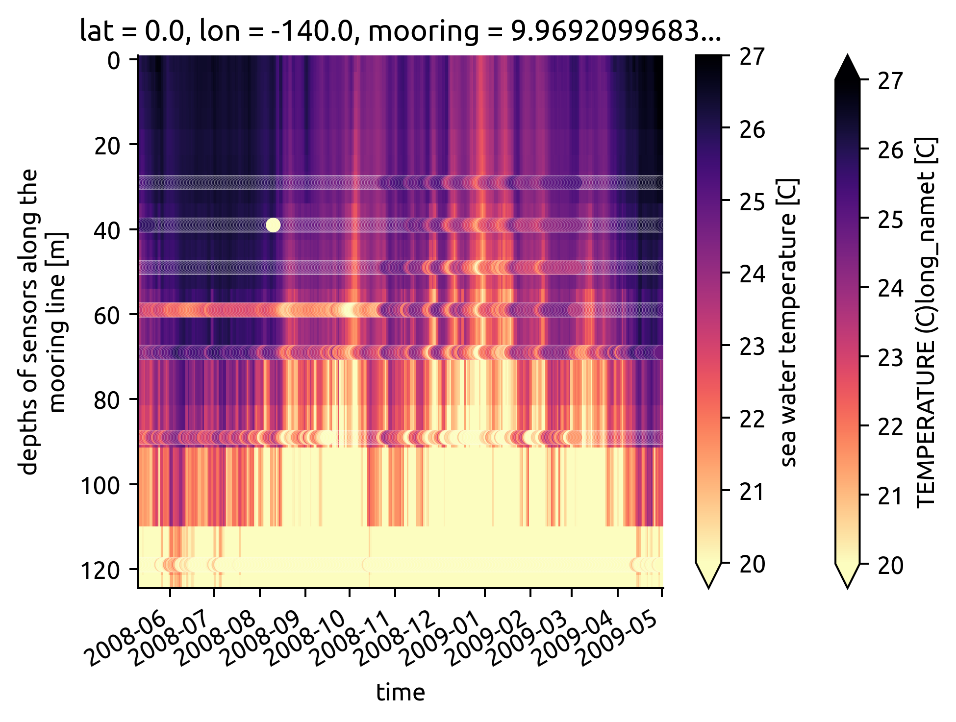
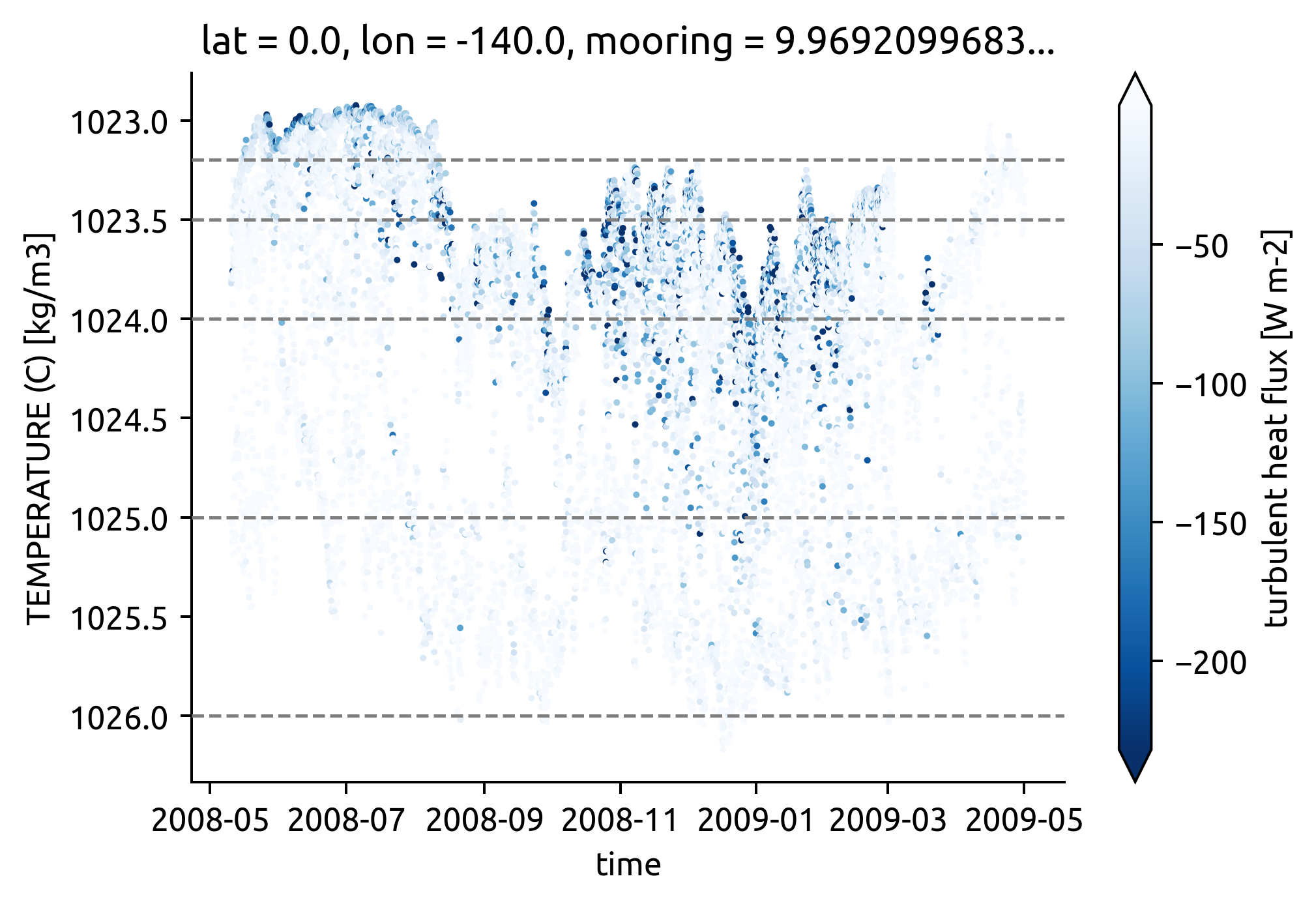
Check for chi T biases
kwargs = dict(vmin=20, vmax=27, cmap=mpl.cm.magma_r)
taos.T.plot(robust=True, yincrease=False, **kwargs)
(
chisub.resample(time="D")
.mean()
.plot.scatter(
**kwargs, y="depth", x="time", hue="T_original", edgecolor="w", linewidth=0.05
)
)
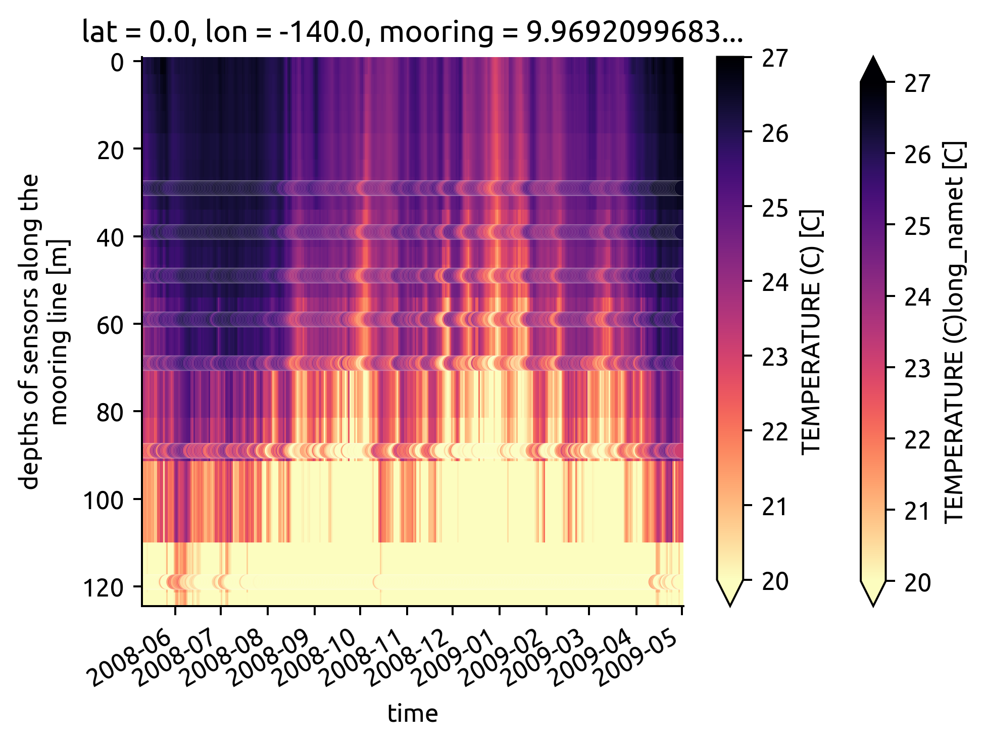
plt.figure()
taos.T.plot(robust=True, yincrease=False, **kwargs)
(
chisub.resample(time="D")
.mean()
.plot.scatter(**kwargs, y="depth", x="time", hue="T", edgecolor="w", linewidth=0.05)
)
<matplotlib.collections.PathCollection at 0x7f10fb34ff10>
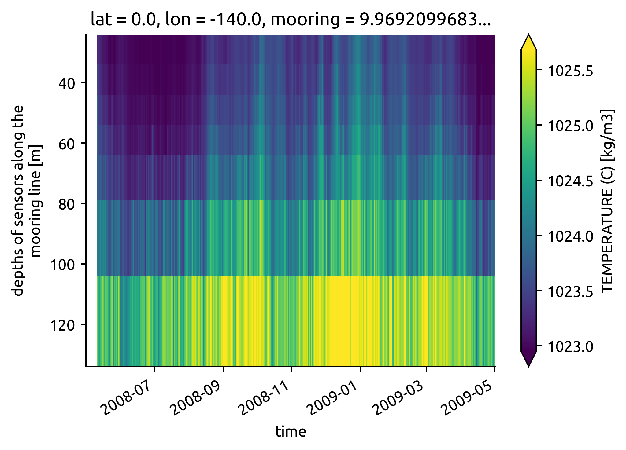
chisub.pden.plot(x="time", yincrease=False, robust=True)
<matplotlib.collections.QuadMesh at 0x7f10fab202b0>
Read in gradients#
argo#
argograd = xr.open_zarr(
    "../datasets/argo_monthly_iso_gradients.zarr", decode_times=False
)
argograd = argograd.cf.guess_coord_axis()
argograd.pres.attrs["positive"] = "down"
argograd = argograd.cf.add_bounds("pres")
argo = (
    argograd.sel(lon=360 + chisub.lon.item(), method="nearest")
    .sel(lat=slice(-3, 8), pres=slice(500))
    .mean("time")
)
argo["pden"] = ed.jmd95.dens(
    argo.Smean, argo.Tmean, 0  # ecco.pres.broadcast_like(ecco.Smean)
)
argo
<xarray.Dataset>
Dimensions:      (bounds: 2, lat: 11, pres: 34)
Coordinates:
  * lat          (lat) float32 -2.5 -1.5 -0.5 0.5 1.5 2.5 3.5 4.5 5.5 6.5 7.5
    lon          float32 220.5
  * pres         (pres) float64 2.5 10.0 20.0 30.0 ... 420.0 440.0 462.5 500.0
    pres_bounds  (bounds, pres) float32 -1.25 6.25 15.0 ... 450.0 473.8 518.8
Dimensions without coordinates: bounds
Data variables:
    Smean        (pres, lat) float32 dask.array<chunksize=(34, 11), meta=np.ndarray>
    Tmean        (pres, lat) float32 dask.array<chunksize=(34, 11), meta=np.ndarray>
    dSdia        (pres, lat) float64 dask.array<chunksize=(34, 11), meta=np.ndarray>
    dSdz         (pres, lat) float32 dask.array<chunksize=(34, 11), meta=np.ndarray>
    dSiso        (pres, lat) float64 dask.array<chunksize=(34, 11), meta=np.ndarray>
    dTdia        (pres, lat) float64 dask.array<chunksize=(34, 11), meta=np.ndarray>
    dTdz         (pres, lat) float32 dask.array<chunksize=(34, 11), meta=np.ndarray>
    dTiso        (pres, lat) float64 dask.array<chunksize=(34, 11), meta=np.ndarray>
    ρmean        (pres, lat) float32 dask.array<chunksize=(34, 11), meta=np.ndarray>
    pden         (pres, lat) float32 dask.array<chunksize=(34, 11), meta=np.ndarray>
Attributes:
    dataset:  argo
name: Mean fields and isopycnal, diapycnal gradients from Argo- bounds: 2
- lat: 11
- pres: 34
- lat(lat)float32-2.5 -1.5 -0.5 0.5 ... 5.5 6.5 7.5
- units :
- degrees_north
- standard_name :
- latitude
- axis :
- Y
- point_spacing :
- even
array([-2.5, -1.5, -0.5, 0.5, 1.5, 2.5, 3.5, 4.5, 5.5, 6.5, 7.5], dtype=float32) - lon()float32220.5
- units :
- degrees_east
- standard_name :
- longitude
- axis :
- X
- modulo :
- 360.0
- point_spacing :
- even
array(220.5, dtype=float32)
- pres(pres)float642.5 10.0 20.0 ... 440.0 462.5 500.0
- axis :
- Z
- point_spacing :
- uneven
- positive :
- down
- units :
- dbar
- bounds :
- pres_bounds
array([ 2.5, 10. , 20. , 30. , 40. , 50. , 60. , 70. , 80. , 90. , 100. , 110. , 120. , 130. , 140. , 150. , 160. , 170. , 182.5, 200. , 220. , 240. , 260. , 280. , 300. , 320. , 340. , 360. , 380. , 400. , 420. , 440. , 462.5, 500. ]) - pres_bounds(bounds, pres)float32-1.25 6.25 15.0 ... 473.8 518.8
- axis :
- Z
- point_spacing :
- uneven
- positive :
- down
- units :
- dbar
array([[ -1.25,   6.25,  15.  ,  25.  ,  35.  ,  45.  ,  55.  ,  65.  ,
         75.  ,  85.  ,  95.  , 105.  , 115.  , 125.  , 135.  , 145.  ,
        155.  , 165.  , 176.25, 191.25, 210.  , 230.  , 250.  , 270.  ,
        290.  , 310.  , 330.  , 350.  , 370.  , 390.  , 410.  , 430.  ,
        451.25, 481.25],
       [  6.25,  13.75,  25.  ,  35.  ,  45.  ,  55.  ,  65.  ,  75.  ,
         85.  ,  95.  , 105.  , 115.  , 125.  , 135.  , 145.  , 155.  ,
        165.  , 175.  , 188.75, 208.75, 230.  , 250.  , 270.  , 290.  ,
        310.  , 330.  , 350.  , 370.  , 390.  , 410.  , 430.  , 450.  ,
        473.75, 518.75]], dtype=float32)
- Smean(pres, lat)float32dask.array<chunksize=(34, 11), meta=np.ndarray>
Array Chunk Bytes 1.50 kB 1.50 kB Shape (34, 11) (34, 11) Count 113 Tasks 1 Chunks Type float32 numpy.ndarray - Tmean(pres, lat)float32dask.array<chunksize=(34, 11), meta=np.ndarray>
Array Chunk Bytes 1.50 kB 1.50 kB Shape (34, 11) (34, 11) Count 113 Tasks 1 Chunks Type float32 numpy.ndarray - dSdia(pres, lat)float64dask.array<chunksize=(34, 11), meta=np.ndarray>
- long_name :
- Diapycnal ∇S
Array Chunk Bytes 2.99 kB 2.99 kB Shape (34, 11) (34, 11) Count 113 Tasks 1 Chunks Type float64 numpy.ndarray - dSdz(pres, lat)float32dask.array<chunksize=(34, 11), meta=np.ndarray>
- long_name :
- dS/dz
Array Chunk Bytes 1.50 kB 1.50 kB Shape (34, 11) (34, 11) Count 113 Tasks 1 Chunks Type float32 numpy.ndarray - dSiso(pres, lat)float64dask.array<chunksize=(34, 11), meta=np.ndarray>
- long_name :
- Along-isopycnal ∇S
Array Chunk Bytes 2.99 kB 2.99 kB Shape (34, 11) (34, 11) Count 113 Tasks 1 Chunks Type float64 numpy.ndarray - dTdia(pres, lat)float64dask.array<chunksize=(34, 11), meta=np.ndarray>
- long_name :
- Diapycnal ∇T
Array Chunk Bytes 2.99 kB 2.99 kB Shape (34, 11) (34, 11) Count 113 Tasks 1 Chunks Type float64 numpy.ndarray - dTdz(pres, lat)float32dask.array<chunksize=(34, 11), meta=np.ndarray>
- long_name :
- dT/dz
Array Chunk Bytes 1.50 kB 1.50 kB Shape (34, 11) (34, 11) Count 113 Tasks 1 Chunks Type float32 numpy.ndarray - dTiso(pres, lat)float64dask.array<chunksize=(34, 11), meta=np.ndarray>
- long_name :
- Along-isopycnal ∇T
Array Chunk Bytes 2.99 kB 2.99 kB Shape (34, 11) (34, 11) Count 113 Tasks 1 Chunks Type float64 numpy.ndarray - ρmean(pres, lat)float32dask.array<chunksize=(34, 11), meta=np.ndarray>
Array Chunk Bytes 1.50 kB 1.50 kB Shape (34, 11) (34, 11) Count 113 Tasks 1 Chunks Type float32 numpy.ndarray - pden(pres, lat)float32dask.array<chunksize=(34, 11), meta=np.ndarray>
Array Chunk Bytes 1.50 kB 1.50 kB Shape (34, 11) (34, 11) Count 316 Tasks 1 Chunks Type float32 numpy.ndarray
- dataset :
- argo
- name :
- Mean fields and isopycnal, diapycnal gradients from Argo
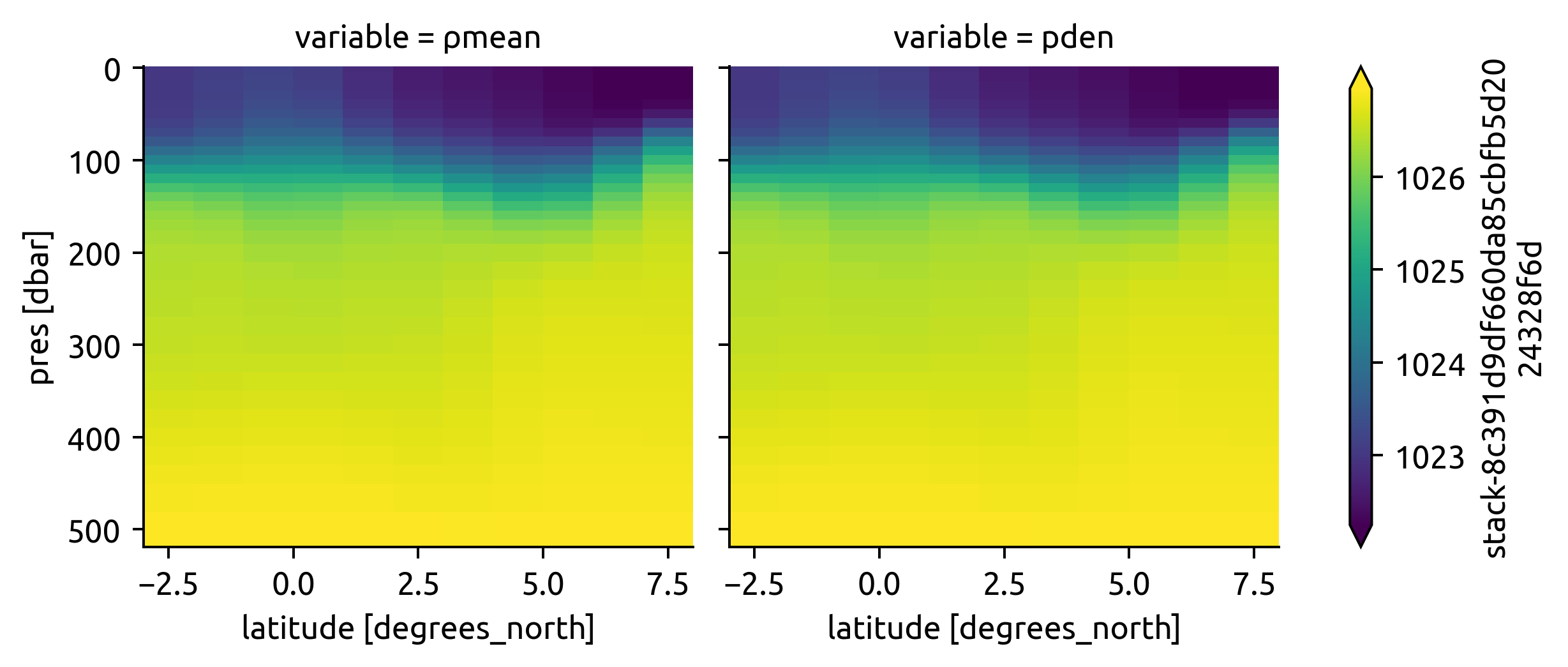
(
    argo[["ρmean", "pden"]]
    # .sel(lon=220, method="nearest")
    .to_array().cf.plot(col="variable", y="vertical", robust=True)
)
<xarray.plot.facetgrid.FacetGrid at 0x7f10fa916c40>
ECCO#
ecco = (
    ed.eddydiff.read_ecco_clim()
    .sel(lon=360 + chisub.lon.item(), method="nearest")
    .sel(lat=slice(-3, 8), pres=slice(500))
    .mean("time")
)
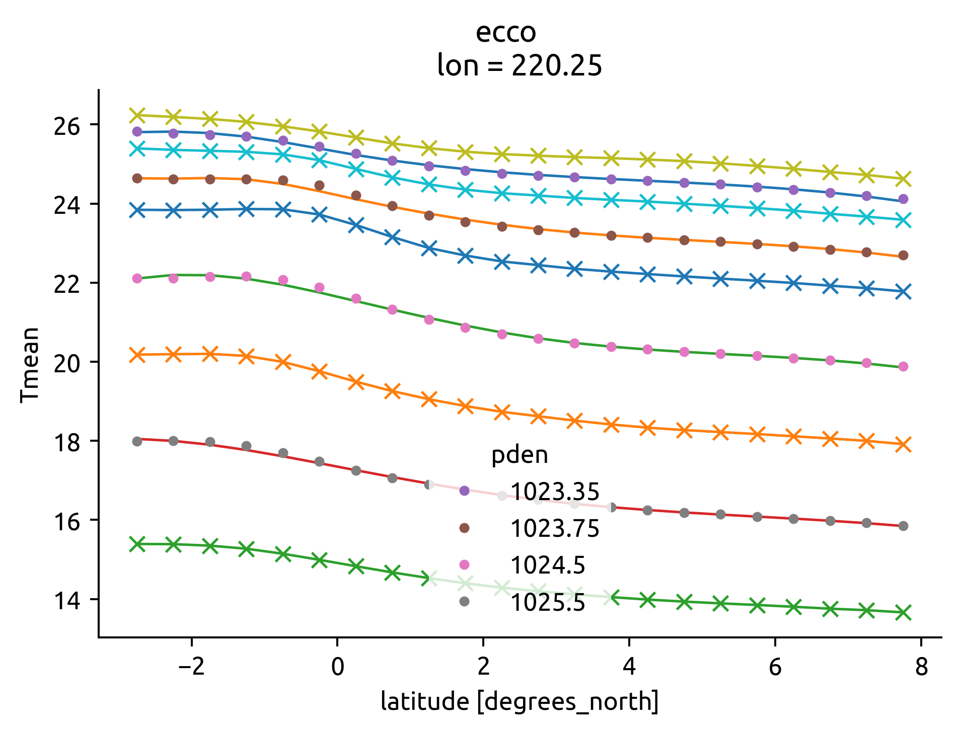
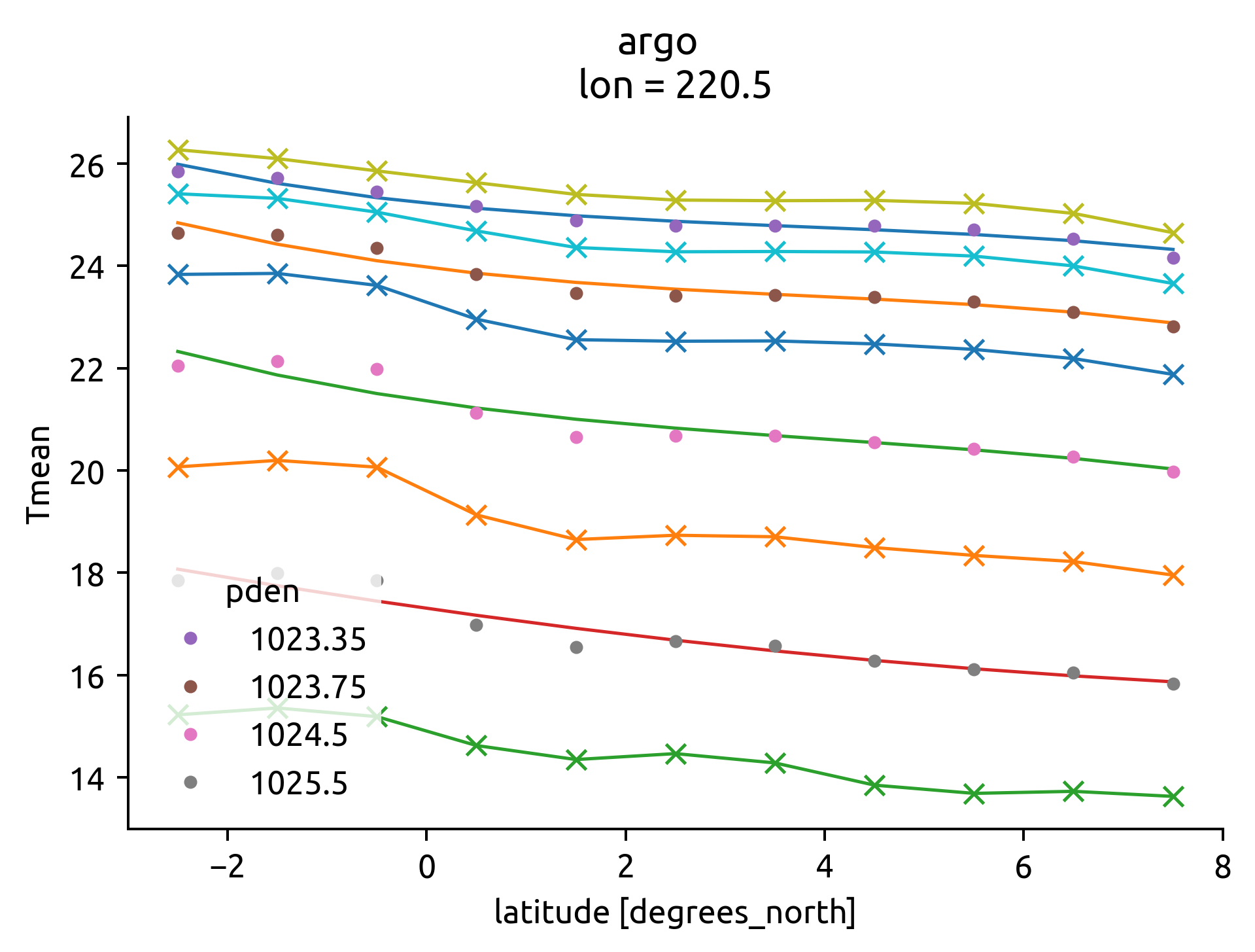
Evaluate bin choices#
How well do ECCO & Argo agree?
Do the chosen ρ levels cross the mooring location? Otherwise I can’t get an estimate of lateral gradient? I need the edges to cross too, so that I can get a vertical gradient
How do the bins look in T-S space? Am I seeing enough stirring to do the analysis
bins = [
1022.5,
1023,
1023.5,
1024,
1024.5,
1025,
1025.5,
1026,
1026.5,
]
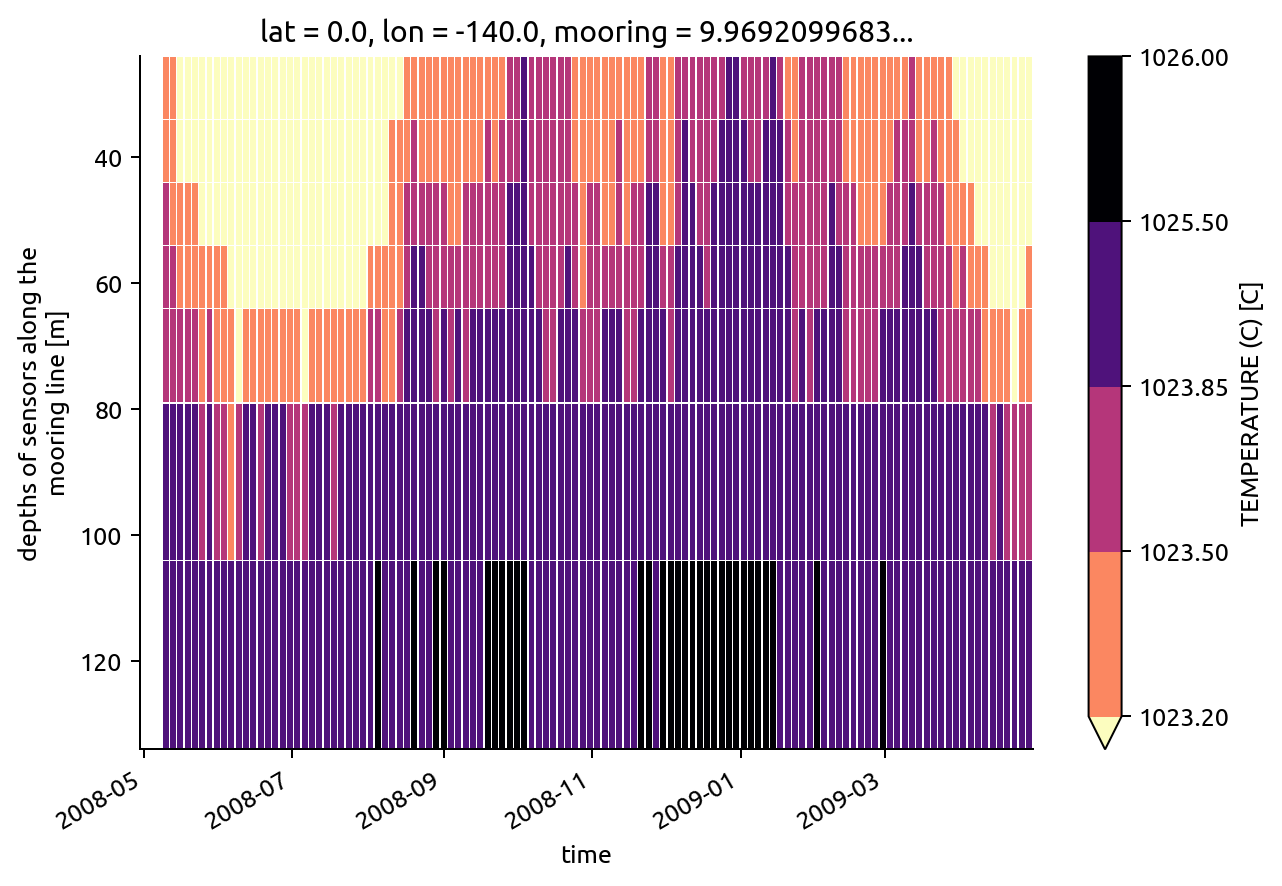
bins = np.array([1023.2, 1023.5, 1024, 1025, 1026])
centers = (bins[1:] + bins[:-1]) / 2
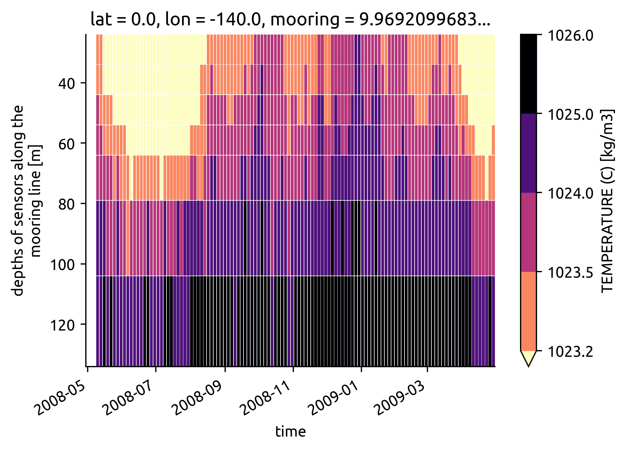
(
chisub.pden.resample(time="3D")
.mean()
.plot(
x="time",
levels=bins,
yincrease=False,
cmap=mpl.cm.magma_r,
edgecolor="w",
linewidths=0.15,
)
)
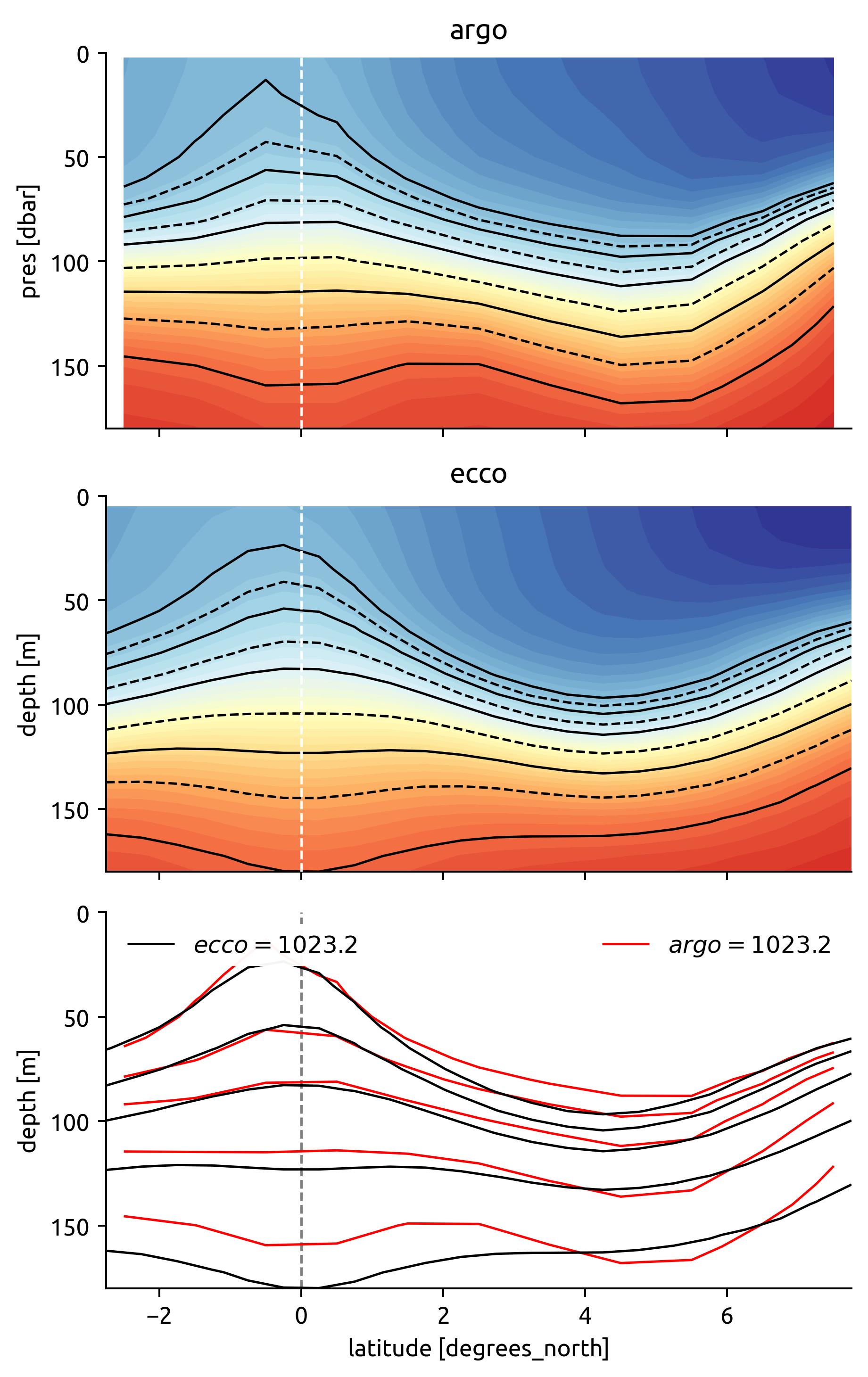
ed.plot.check_bins_with_climatology(bins, argo, ecco)
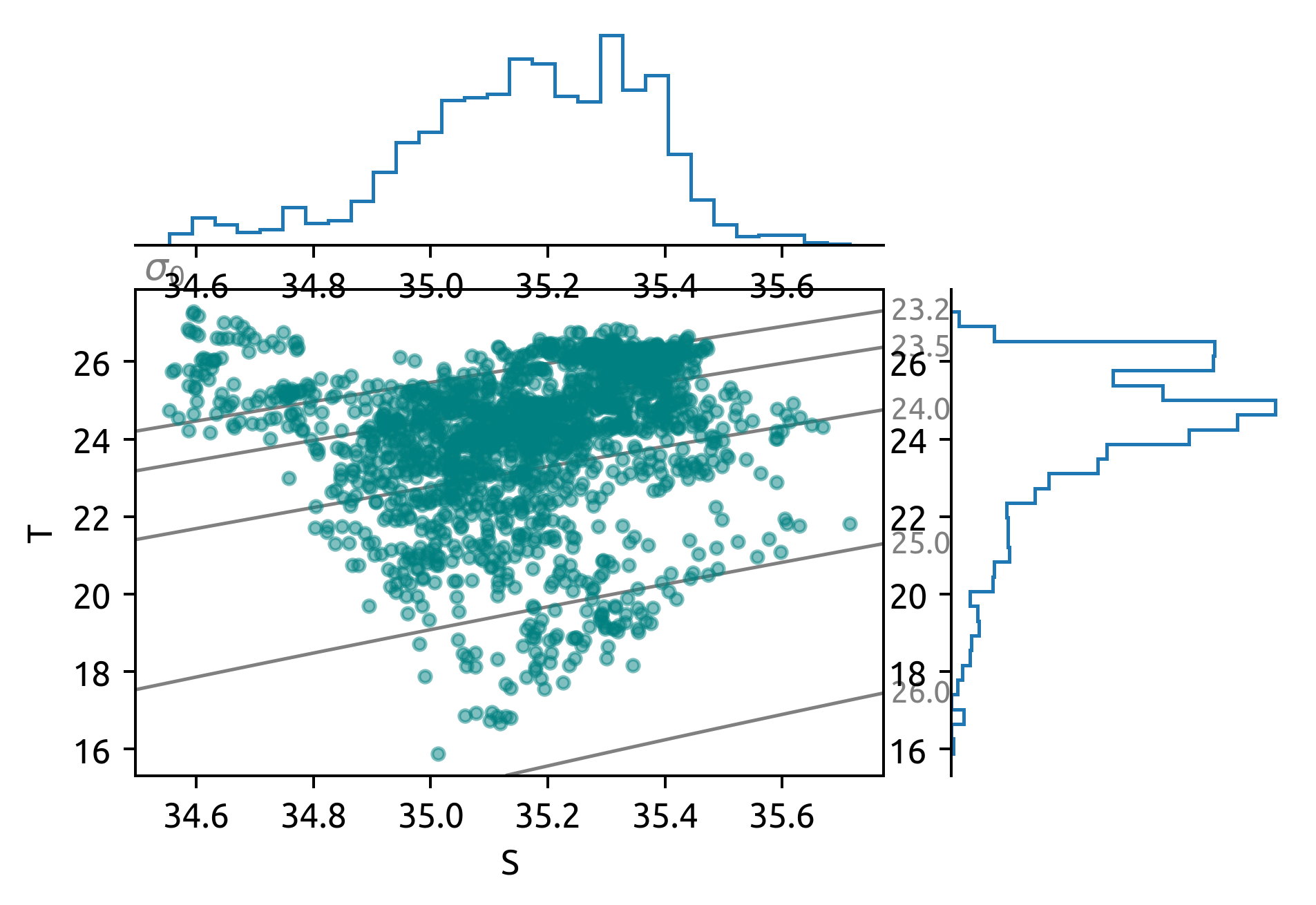
dcpy.oceans.TSplot(
taos.S,
taos.T,
rho_levels=bins,
hexbin=False,
)
# chi to density space
plt.figure()
chisub.plot.scatter(x="time", y="pden", hue="Jq", robust=True, cmap=mpl.cm.Blues_r, s=1)
plt.gca().yaxis.set_inverted(True)
if "bins" in locals():
dcpy.plots.liney(bins, zorder=10)
/home/deepak/work/python/dcpy/dcpy/plots.py:1006: MatplotlibDeprecationWarning:
The ax attribute was deprecated in Matplotlib 3.3 and will be removed two minor releases later.
  ax = cs.ax
/home/deepak/miniconda3/envs/dcpy/lib/python3.8/site-packages/IPython/core/pylabtools.py:132: UserWarning: constrained_layout not applied.  At least one axes collapsed to zero width or height.
  fig.canvas.print_figure(bytes_io, **kw)
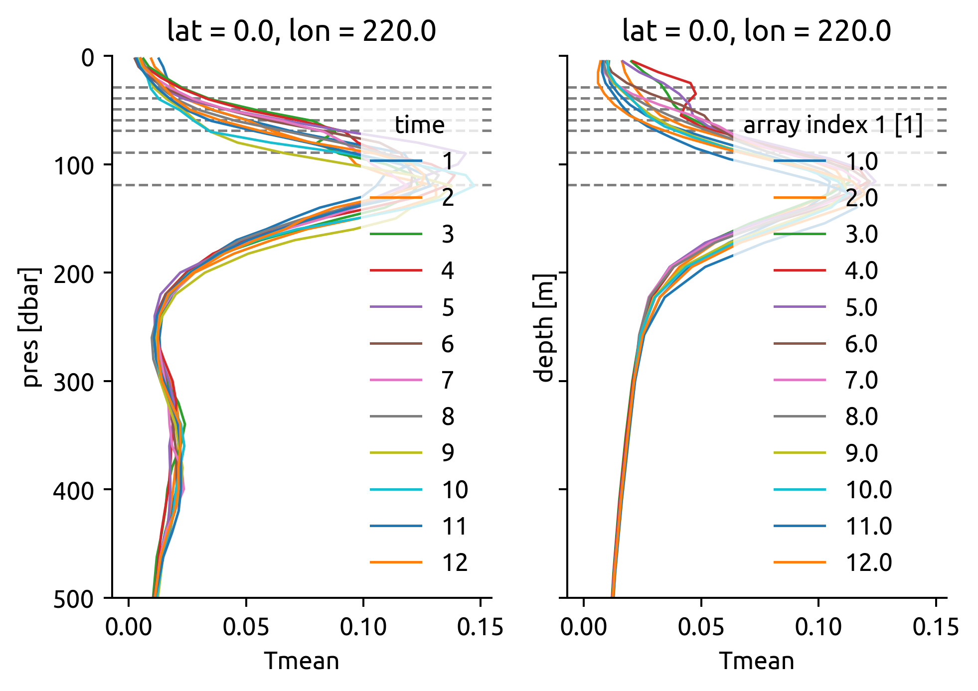
Compare dTdz between mean field and mooring#
f, ax = plt.subplots(1, 2, sharex=True, sharey=True)
(
    (-1 * argograd.Tmean.interp(lat=chisub.lat.values, lon=360 + chisub.lon.values))
    .differentiate("pres")
    .cf.plot(y="Z", ylim=(500, 0), hue="time", ax=ax[0])
)


(
    (
        -1
        * eccograd.drop("dayofyear").Tmean.interp(
            lat=chisub.lat.values, lon=360 + chisub.lon.values
        )
    )
    .differentiate("pres")
    .cf.plot(y="Z", ylim=(500, 0), hue="time", ax=ax[1])
)

[dcpy.plots.liney(chisub.depth, ax=aa) for aa in ax]

# eccoT["dTdz"].sel(lat=0, method="nearest").plot(y="z")
[None, None]
Do estimate#
eccoT, edge = ed.eddydiff.estimate_gradients(ecco, bins, debug=True)
argoT, edge = ed.eddydiff.estimate_gradients(argo, bins, debug=True)
# .sel(depth=slice(39, None))  # TODO: wintertime MLD?
chidens = ed.eddydiff.bin_avg_in_density_time(
    chisub.reset_coords(drop=True).where(chisub.KT < 1e-3).coarsen(time=24).mean(),
    bins={"pden": bins},
)
chidens
<xarray.Dataset>
Dimensions:             (binvar: 4, time: 13)
Coordinates:
  * binvar              (binvar) float64 1.023e+03 1.024e+03 1.024e+03 1.026e+03
  * time                (time) datetime64[ns] 2008-05-01 ... 2009-05-01
Data variables: (12/16)
    depth               (binvar, time) float64 57.4 69.0 69.0 ... 119.0 nan
    T_original          (binvar, time) float64 23.86 24.56 25.29 ... 17.92 nan
    dTdz                (binvar, time) float64 0.04416 0.06119 ... 0.1247 nan
    N2                  (binvar, time) float64 0.0001219 0.0001575 ... nan
    KT                  (binvar, time) float64 9.291e-05 4.81e-05 ... nan
    chi                 (binvar, time) float64 1.76e-07 2.496e-07 ... nan
    ...                  ...
    lat                 (binvar, time) float64 0.0 0.0 0.0 0.0 ... 0.0 0.0 nan
    lon                 (binvar, time) float64 -140.0 -140.0 ... -140.0 nan
    mooring             (binvar, time) float64 9.969e+36 9.969e+36 ... nan
    chipod              (binvar, time) float64 9.969e+36 9.969e+36 ... nan
    reference_pressure  (binvar, time) float64 0.0 0.0 0.0 0.0 ... 0.0 0.0 nan
numobs (binvar, time) float64 25.0 33.0 23.0 ... 31.0 13.0 nan- binvar: 4
- time: 13
- binvar(binvar)float641.023e+03 1.024e+03 ... 1.026e+03
array([1023.35, 1023.75, 1024.5 , 1025.5 ])
- time(time)datetime64[ns]2008-05-01 ... 2009-05-01
array(['2008-05-01T00:00:00.000000000', '2008-06-01T00:00:00.000000000',
       '2008-07-01T00:00:00.000000000', '2008-08-01T00:00:00.000000000',
       '2008-09-01T00:00:00.000000000', '2008-10-01T00:00:00.000000000',
       '2008-11-01T00:00:00.000000000', '2008-12-01T00:00:00.000000000',
       '2009-01-01T00:00:00.000000000', '2009-02-01T00:00:00.000000000',
       '2009-03-01T00:00:00.000000000', '2009-04-01T00:00:00.000000000',
       '2009-05-01T00:00:00.000000000'], dtype='datetime64[ns]')
- depth(binvar, time)float6457.4 69.0 69.0 ... 119.0 119.0 nan
array([[ 57.4 , 69. , 69. , 63. , nan, 38.09090909, 35.66666667, 37.125 , 36.5 , 39.22727273, 39. , 69. , 69. ], [ 69.66666667, 88.16666667, 85.36363636, 64.625 , 62.77777778, 62.40909091, 53.49275362, 44.27777778, 43.58823529, 52.17073171, 67.125 , 69. , nan], [111.5 , 114.86206897, 113.23076923, 82.63636364, 76. , 83.28571429, 80.53846154, 62.7804878 , 69.46511628, 80.42857143, 71.85714286, 116.22222222, 119. ], [119. , 119. , 119. , 119. , 119. , 119. , 117.88888889, 108.56521739, 115.47058824, 117.92857143, 119. , 119. , nan]]) - T_original(binvar, time)float6423.86 24.56 25.29 ... 17.92 nan
array([[23.85671815, 24.56274384, 25.29199903, 23.41170561, nan, 24.90510844, 24.93044712, 24.78918144, 24.53358385, 24.33838055, 24.40988869, 25.14286602, 24.81364424], [23.66386686, 23.51252827, 23.75645903, 22.45411171, 22.27486304, 22.77676902, 23.87536426, 23.68775554, 23.45761806, 23.85152579, 23.62878343, 24.02487077, nan], [19.94920734, 20.50231554, 19.95847035, 21.24291699, 21.73389625, 20.85695274, 21.68110843, 21.67157252, 21.6548754 , 21.77154881, 22.05744945, 19.64100105, 18.43640687], [18.10242429, 18.01367236, 18.12910808, 17.06256153, 16.50716736, 17.56813041, 17.34387361, 16.74562503, 17.00604839, 17.29050379, 17.31957765, 17.92119601, nan]]) - dTdz(binvar, time)float640.04416 0.06119 ... 0.1247 nan
array([[0.04416214, 0.06118726, 0.07297678, 0.05801599, nan, 0.01473227, 0.02566456, 0.02618847, 0.0272221 , 0.02021343, 0.03801468, 0.06142622, 0.06508826], [0.06086953, 0.08836653, 0.10837099, 0.07754813, 0.07090517, 0.04433695, 0.0536134 , 0.04277092, 0.03704573, 0.03837401, 0.07294284, 0.08321904, nan], [0.12091924, 0.11239624, 0.12956577, 0.09833623, 0.10854905, 0.08778405, 0.09155011, 0.08349398, 0.07180119, 0.10497851, 0.09564591, 0.14178686, 0.16689607], [0.12329707, 0.15328839, 0.1222167 , 0.12626973, 0.09541173, 0.09510892, 0.10337439, 0.1109687 , 0.10390768, 0.10760278, 0.0976528 , 0.12468748, nan]]) - N2(binvar, time)float640.0001219 0.0001575 ... nan
array([[1.21852364e-04, 1.57502209e-04, 1.88671136e-04, 1.51144707e-04, nan, 3.21534147e-05, 6.72968133e-05, 5.70370484e-05, 6.17608141e-05, 5.68115761e-05, 9.86899156e-05, 1.65410840e-04, 1.66742451e-04], [1.58983950e-04, 2.17185338e-04, 2.58588103e-04, 1.82884337e-04, 1.67043259e-04, 1.00472258e-04, 1.16125844e-04, 8.24007967e-05, 9.46934685e-05, 9.60004989e-05, 1.76139389e-04, 2.02670024e-04, nan], [2.83181589e-04, 2.70318910e-04, 3.12337523e-04, 2.24221808e-04, 2.56636017e-04, 2.07142672e-04, 2.17488457e-04, 1.77748147e-04, 1.77327819e-04, 2.41577285e-04, 2.29421208e-04, 3.36845877e-04, 3.91854544e-04], [2.70247672e-04, 3.43166965e-04, 2.74589152e-04, 2.80604465e-04, 2.11146932e-04, 2.15989813e-04, 2.34673634e-04, 2.43970665e-04, 2.32542184e-04, 2.42580131e-04, 2.21181098e-04, 2.87844531e-04, nan]]) - KT(binvar, time)float649.291e-05 4.81e-05 ... nan
array([[9.29117650e-05, 4.81039215e-05, 9.50149549e-05, 1.84934243e-04, nan, 4.64265937e-04, 3.07736722e-04, 2.56670772e-04, 3.14299542e-04, 2.69522271e-04, 4.28721997e-05, 2.86556182e-05, 7.74815593e-06], [6.96865990e-05, 4.55297786e-05, 7.67445150e-05, 1.24871827e-04, 9.96037295e-05, 2.41893612e-04, 2.08132286e-04, 2.08839577e-04, 2.54144302e-04, 1.78177247e-04, 4.98799211e-05, 2.47024134e-05, nan], [3.63189972e-05, 5.28758150e-05, 6.64222760e-05, 3.42939464e-05, 1.05926874e-04, 8.55479829e-05, 1.02924463e-04, 1.09738642e-04, 8.25417823e-05, 5.05339137e-05, 3.23275368e-05, 8.31044721e-05, 8.87949896e-05], [7.97119582e-05, 1.08046467e-04, 1.09167204e-04, 9.19962199e-05, 8.91138843e-05, 1.01928983e-04, 1.04267559e-04, 7.21110633e-05, 9.31272959e-05, 1.07583409e-04, 1.08438187e-04, 1.00424004e-04, nan]]) - chi(binvar, time)float641.76e-07 2.496e-07 ... nan
- long_name :
- $χ$
array([[1.76045240e-07, 2.49612344e-07, 8.68468335e-07, 6.98716890e-07, nan, 1.26478939e-07, 2.77384463e-07, 1.65624606e-07, 1.85511228e-07, 9.76086514e-08, 4.47917178e-08, 4.28343991e-08, 2.26248616e-09], [9.42690766e-08, 2.05087568e-07, 7.39229616e-07, 8.27983766e-07, 6.26312789e-07, 7.95233806e-07, 8.13019603e-07, 2.63485722e-07, 4.59532497e-07, 2.60225103e-07, 4.86839636e-07, 1.86891081e-07, nan], [1.92647830e-08, 1.17063084e-07, 9.95941976e-08, 2.21797645e-07, 1.23803315e-06, 6.15444592e-07, 1.26277666e-06, 1.00097521e-06, 6.04342353e-07, 6.02153333e-07, 3.81056898e-07, 2.90401978e-08, 1.44412199e-08], [1.64444059e-08, 1.39925573e-07, 7.34096008e-08, 2.13509428e-07, 5.23514966e-08, 1.48479192e-07, 5.35569827e-08, 6.89204834e-07, 1.29493150e-07, 5.18768392e-08, 5.07705981e-08, 3.50184439e-08, nan]]) - eps(binvar, time)float643.303e-08 2.838e-08 ... nan
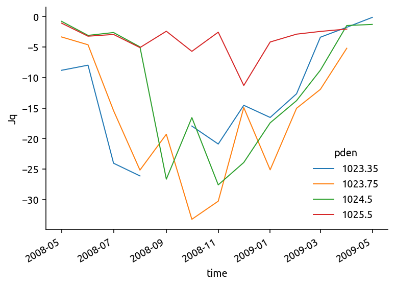
array([[3.30292013e-08, 2.83757015e-08, 8.49390607e-08, 9.86640835e-08, nan, 6.07467838e-08, 7.78271835e-08, 5.20021646e-08, 5.64751639e-08, 5.22195283e-08, 1.38002503e-08, 6.92040276e-09, 5.71766855e-10], [1.31557494e-08, 1.60867317e-08, 5.29659381e-08, 8.62587316e-08, 6.38309258e-08, 1.10006569e-07, 9.82530190e-08, 5.09384241e-08, 9.35435009e-08, 5.70937441e-08, 3.91630764e-08, 1.70262490e-08, nan], [3.26604043e-09, 1.15136021e-08, 1.11962978e-08, 1.59902878e-08, 8.80443112e-08, 5.80034254e-08, 9.44214840e-08, 7.28517335e-08, 6.19610666e-08, 4.37851010e-08, 2.80970409e-08, 5.57078046e-09, 6.16431309e-09], [3.70431120e-09, 1.10955727e-08, 1.54000192e-08, 1.68602242e-08, 8.37346332e-09, 1.86276832e-08, 8.54768728e-09, 3.53329777e-08, 1.55705266e-08, 1.05566558e-08, 8.43822472e-09, 7.55966982e-09, nan]]) - Jq(binvar, time)float64-8.807 -7.973 -24.03 ... -2.053 nan
array([[ -8.80739164, -7.97338511, -24.03147417, -26.10804168, nan, -17.94441252, -20.88567984, -14.54247042, -16.53562888, -12.6606896 , -3.39373812, -1.76632801, -0.14510847], [ -3.35552511, -4.63217733, -15.4218806 , -25.15439722, -19.28951314, -33.21501913, -30.24583221, -14.91146921, -25.10889353, -15.03611923, -11.93251869, -5.20015281, nan], [ -0.79609946, -3.09462011, -2.62713362, -4.97481365, -26.64153322, -16.55948177, -27.57749243, -23.91079199, -17.41701104, -13.78064065, -8.79289719, -1.47945808, -1.29364761], [ -1.0950149 , -3.22645576, -2.94163398, -5.09216929, -2.41281222, -5.70714109, -2.56850569, -11.29964097, -4.17654176, -2.89137245, -2.44390353, -2.05286118, nan]]) - KtTz(binvar, time)float643.559e-06 2.792e-06 ... nan
- long_name :
- $⟨K_T T_z⟩$
array([[3.55922951e-06, 2.79166159e-06, 6.73691091e-06, 8.67942951e-06, nan, 6.20933088e-06, 6.82133025e-06, 4.93159407e-06, 6.68587593e-06, 4.20386412e-06, 1.21333784e-06, 1.15379973e-06, 4.14527700e-07], [2.54526096e-06, 3.43141996e-06, 7.53488932e-06, 7.84798670e-06, 6.24579243e-06, 9.35951412e-06, 9.84329877e-06, 6.23045357e-06, 7.80438258e-06, 5.45613587e-06, 3.65958196e-06, 1.99425418e-06, nan], [3.62020274e-06, 4.53471425e-06, 7.19284015e-06, 3.39332171e-06, 8.61579746e-06, 6.93235767e-06, 9.80662010e-06, 7.69785848e-06, 5.54208762e-06, 5.05506257e-06, 2.99317947e-06, 1.02225139e-05, 1.43220384e-05], [7.37630188e-06, 1.53415873e-05, 1.25653364e-05, 1.03990392e-05, 8.21498044e-06, 7.79420605e-06, 1.01393480e-05, 7.73687251e-06, 9.07756535e-06, 1.10452390e-05, 1.00253722e-05, 1.30111558e-05, nan]]) - T(binvar, time)float6424.94 25.0 25.1 ... 17.64 18.38 nan
array([[24.94462026, 25.00148261, 25.10329355, 24.91057913, nan, 24.82142651, 24.82484748, 24.84969283, 24.75621387, 24.73247762, 24.88489974, 25.04744331, 24.74242501], [23.92225586, 23.47843093, 23.68947263, 23.59896831, 23.62926037, 23.50137123, 23.81116079, 23.68802759, 23.56200523, 23.81678247, 23.49269053, 23.97107873, nan], [20.44534525, 20.8331178 , 20.42378494, 21.45172113, 21.85322309, 21.17783388, 21.26756695, 21.47272974, 21.45899408, 21.36650296, 21.93480184, 20.2512622 , 19.19403752], [18.63793704, 18.58231194, 18.53821576, 17.60478415, 16.90785293, 17.94285066, 17.6552955 , 16.75465454, 17.29491573, 17.62587205, 17.64209653, 18.38016743, nan]]) - lat(binvar, time)float640.0 0.0 0.0 0.0 ... 0.0 0.0 0.0 nan
array([[ 0., 0., 0., 0., nan, 0., 0., 0., 0., 0., 0., 0., 0.], [ 0., 0., 0., 0., 0., 0., 0., 0., 0., 0., 0., 0., nan], [ 0., 0., 0., 0., 0., 0., 0., 0., 0., 0., 0., 0., 0.], [ 0., 0., 0., 0., 0., 0., 0., 0., 0., 0., 0., 0., nan]]) - lon(binvar, time)float64-140.0 -140.0 -140.0 ... -140.0 nan
array([[-140., -140., -140., -140., nan, -140., -140., -140., -140., -140., -140., -140., -140.], [-140., -140., -140., -140., -140., -140., -140., -140., -140., -140., -140., -140., nan], [-140., -140., -140., -140., -140., -140., -140., -140., -140., -140., -140., -140., -140.], [-140., -140., -140., -140., -140., -140., -140., -140., -140., -140., -140., -140., nan]]) - mooring(binvar, time)float649.969e+36 9.969e+36 ... nan
array([[9.96920997e+36, 9.96920997e+36, 9.96920997e+36, 9.96920997e+36, nan, 9.96920997e+36, 9.96920997e+36, 9.96920997e+36, 9.96920997e+36, 9.96920997e+36, 9.96920997e+36, 9.96920997e+36, 9.96920997e+36], [9.96920997e+36, 9.96920997e+36, 9.96920997e+36, 9.96920997e+36, 9.96920997e+36, 9.96920997e+36, 9.96920997e+36, 9.96920997e+36, 9.96920997e+36, 9.96920997e+36, 9.96920997e+36, 9.96920997e+36, nan], [9.96920997e+36, 9.96920997e+36, 9.96920997e+36, 9.96920997e+36, 9.96920997e+36, 9.96920997e+36, 9.96920997e+36, 9.96920997e+36, 9.96920997e+36, 9.96920997e+36, 9.96920997e+36, 9.96920997e+36, 9.96920997e+36], [9.96920997e+36, 9.96920997e+36, 9.96920997e+36, 9.96920997e+36, 9.96920997e+36, 9.96920997e+36, 9.96920997e+36, 9.96920997e+36, 9.96920997e+36, 9.96920997e+36, 9.96920997e+36, 9.96920997e+36, nan]]) - chipod(binvar, time)float649.969e+36 9.969e+36 ... nan
array([[9.96920997e+36, 9.96920997e+36, 9.96920997e+36, 9.96920997e+36, nan, 9.96920997e+36, 9.96920997e+36, 9.96920997e+36, 9.96920997e+36, 9.96920997e+36, 9.96920997e+36, 9.96920997e+36, 9.96920997e+36], [9.96920997e+36, 9.96920997e+36, 9.96920997e+36, 9.96920997e+36, 9.96920997e+36, 9.96920997e+36, 9.96920997e+36, 9.96920997e+36, 9.96920997e+36, 9.96920997e+36, 9.96920997e+36, 9.96920997e+36, nan], [9.96920997e+36, 9.96920997e+36, 9.96920997e+36, 9.96920997e+36, 9.96920997e+36, 9.96920997e+36, 9.96920997e+36, 9.96920997e+36, 9.96920997e+36, 9.96920997e+36, 9.96920997e+36, 9.96920997e+36, 9.96920997e+36], [9.96920997e+36, 9.96920997e+36, 9.96920997e+36, 9.96920997e+36, 9.96920997e+36, 9.96920997e+36, 9.96920997e+36, 9.96920997e+36, 9.96920997e+36, 9.96920997e+36, 9.96920997e+36, 9.96920997e+36, nan]]) - reference_pressure(binvar, time)float640.0 0.0 0.0 0.0 ... 0.0 0.0 0.0 nan
array([[ 0., 0., 0., 0., nan, 0., 0., 0., 0., 0., 0., 0., 0.], [ 0., 0., 0., 0., 0., 0., 0., 0., 0., 0., 0., 0., nan], [ 0., 0., 0., 0., 0., 0., 0., 0., 0., 0., 0., 0., 0.], [ 0., 0., 0., 0., 0., 0., 0., 0., 0., 0., 0., 0., nan]]) - numobs(binvar, time)float6425.0 33.0 23.0 ... 31.0 13.0 nan
array([[25., 33., 23., 20., nan, 11., 39., 16., 12., 44.,  9., 15.,  1.],
       [30., 24., 22., 32., 45., 44., 69., 72., 85., 82., 16., 10., nan],
       [20., 29., 26., 11., 20., 35., 52., 82., 86., 42., 21., 18.,  1.],
       [ 7.,  5., 10., 28., 28., 22., 27., 46., 34., 28., 31., 13., nan]])
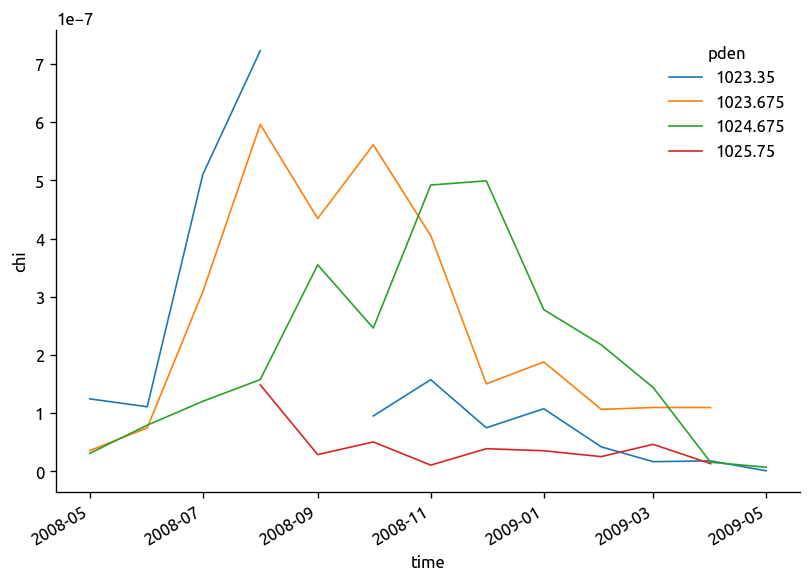
%matplotlib inline
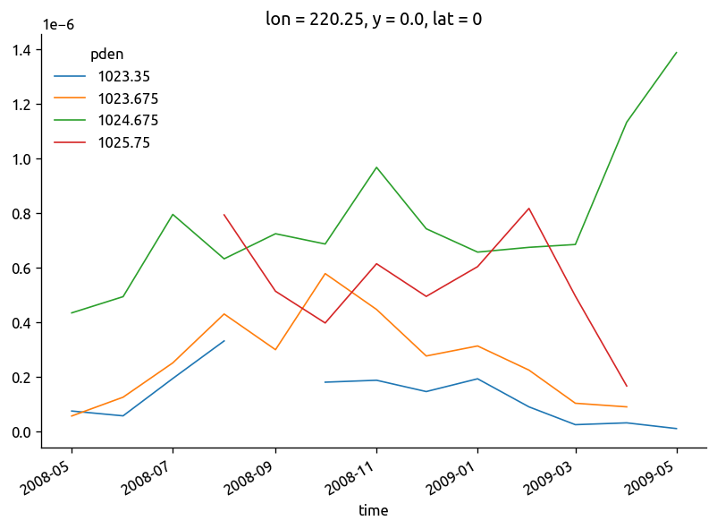
chidens.Jq.plot.line(hue="pden")
[<matplotlib.lines.Line2D at 0x7f10faba7460>,
 <matplotlib.lines.Line2D at 0x7f10e0373d90>,
 <matplotlib.lines.Line2D at 0x7f10b09c0280>,
 <matplotlib.lines.Line2D at 0x7f10b09c01c0>]
%matplotlib inline
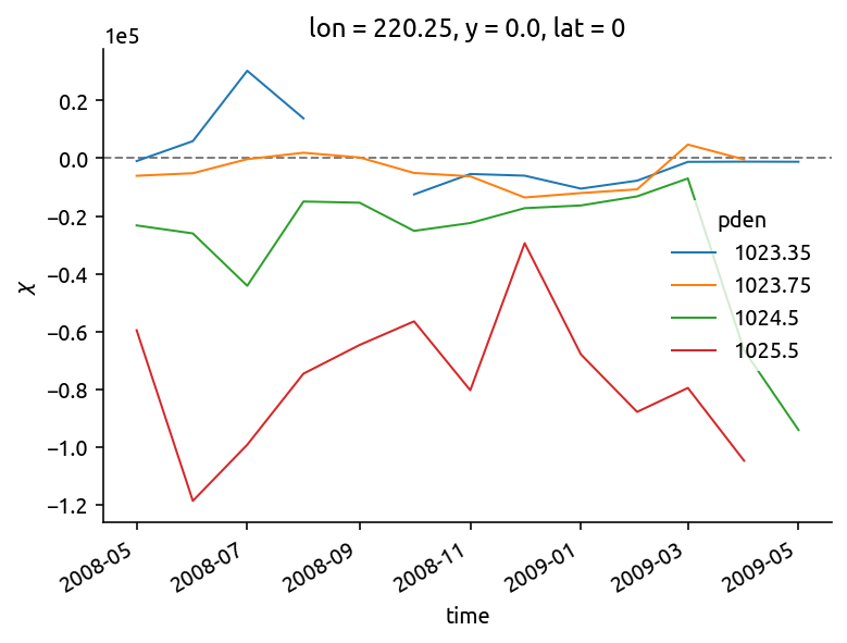
isoT = eccoT.interp(lat=0)
Ke = (chidens["chi"] / 2 - (chidens["KtTz"] * isoT["dTdz"])) / (isoT["dTdy"] ** 2)
Ke.plot.line(hue="pden")
dcpy.plots.liney(0)
Debugging estimate#
Seasonal cycle in ‘inverse” \(T_z\) estimated as \(⟨χ/2⟩ / ⟨K_T T_z⟩\)
Negative \(K_e\) values are where the annual mean gradient in climatology is larger than the “inverse” \(T_z\)
\(⟨T^χ_z⟩\) from χpods averaged in density space is always larger than the other two estimates
%matplotlib inline

est = chidens.isel(pden=2)
isoTz = isoT.dTdz.isel(pden=2)

f, axx = plt.subplots(
    4,
    1,
    sharex=True,
    sharey=False,
    squeeze=False,
    constrained_layout=True,
    figsize=(4, 6),
)
ax = dict(zip(["count", "chi", "KtTz", "Tz"], axx.flat))

(est["numobs"]).plot.step(ax=ax["count"])
(est.chi / 2).plot.step(ax=ax["chi"], label="$⟨χ/2⟩$")
(est.KtTz * isoTz).plot.step(ax=ax["chi"], label="$⟨K_T T_z⟩ ⟨T_z⟩$", _labels=False)
ax["chi"].legend()
# (est.KtTz * est.dTdz).plot(ax=ax["chi"])

(est.KtTz).plot.step(ax=ax["KtTz"])

(est.dTdz).plot.step(ax=ax["Tz"], label="$⟨T^χ_z⟩$")
(est.chi / 2 / est.KtTz).plot.step(
    ax=ax["Tz"], label="$⟨χ/2⟩ / ⟨K_T T_z⟩$", _labels=False
)
dcpy.plots.liney(isoTz, ax=ax["Tz"], label="$⟨T_z⟩$")
ax["Tz"].legend()
dcpy.plots.clean_axes(axx)
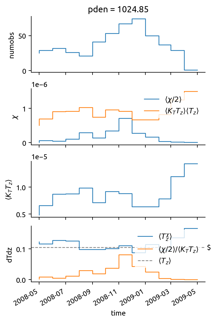
The “seasonal” cycle in \(T_z\) is funny. There are more observations being averaged over and those observations are at 30,40,50m.
I thought it is an artifact. BUT what if there is a seasonal cycle in \(T_z\) in in the isopycnal bins.
In depth space, \(T_z\) increases with depth, so if the isopycnal surface shallows for two months (DJF here), “effective” dT/dz is smaller than our climatological estimate. This ends up being negative \(K_e\)
I think this is being ignored in the equations. Maybe this is advection at “eddy” timescales that is changing \(T_z\) at the “eddy” timescale
Manually excluding everything above 59m improves things a bunch.
Things that may help:
Choose bins to avoid this by looking at plots?
add a diagnostic that checks for scatter in \(T_z\) in chosen bins. This could help with 1.
Explicitly account for this as a source of variance?
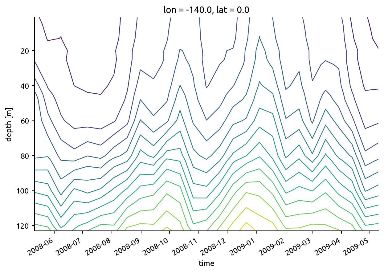
taos.rhoT.resample(time="2W").mean().plot.contour(levels=20, yincrease=False)
<matplotlib.contour.QuadContourSet at 0x7fa71984b110>
(
    chisub.pden.resample(time="3D")
    .mean()
    .plot(
        x="time",
        levels=bins,
        yincrease=False,
        cmap=mpl.cm.magma_r,
        edgecolor="w",
        linewidths=0.15,
    )
)
<matplotlib.collections.QuadMesh at 0x7fa71d96e750>
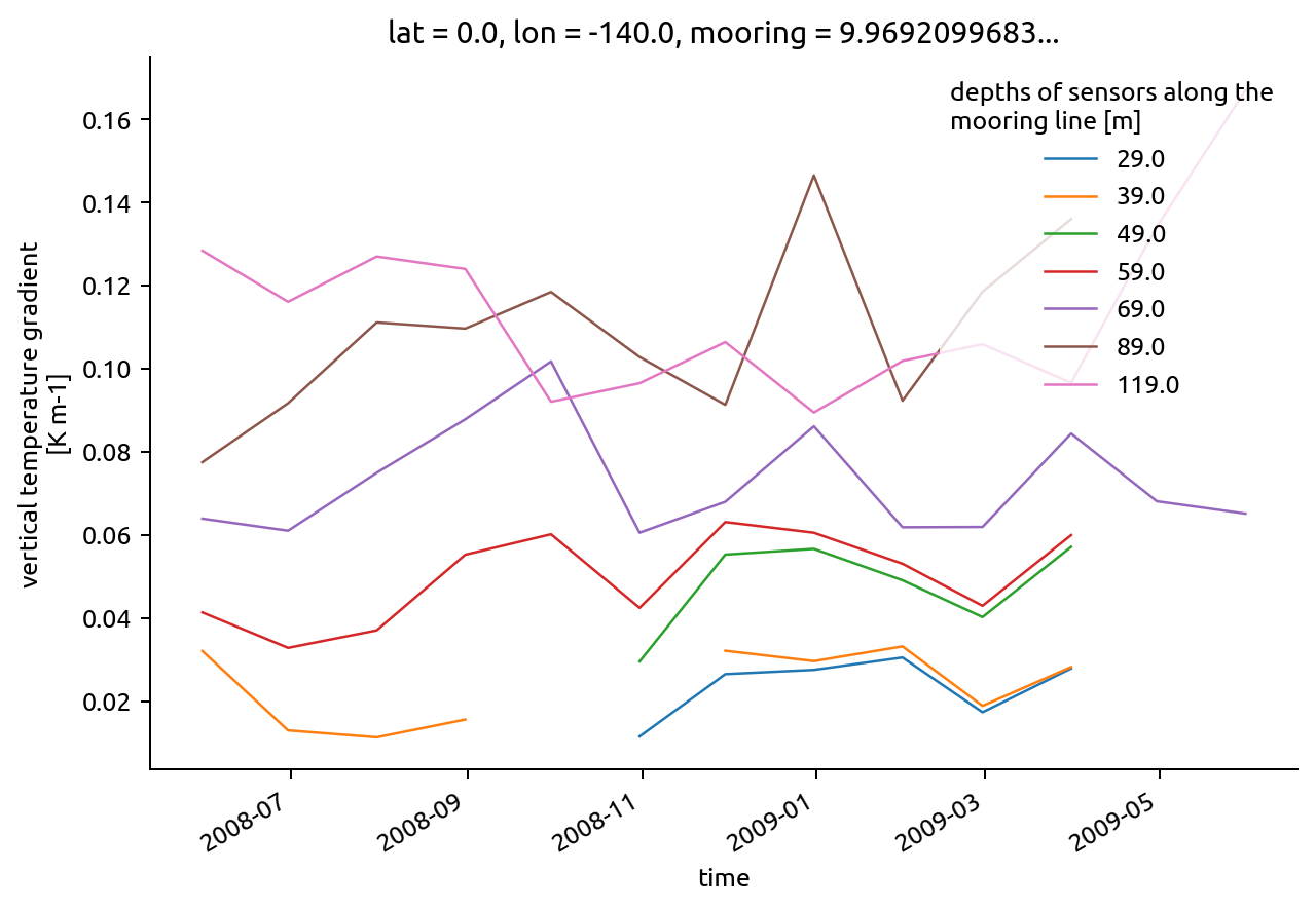
chisub.resample(time="M").mean().dTdz.plot.line(hue="depth")
[<matplotlib.lines.Line2D at 0x7fa719870cd0>,
 <matplotlib.lines.Line2D at 0x7fa71636d390>,
 <matplotlib.lines.Line2D at 0x7fa7197d9dd0>,
 <matplotlib.lines.Line2D at 0x7fa7197cd850>,
 <matplotlib.lines.Line2D at 0x7fa716323650>,
 <matplotlib.lines.Line2D at 0x7fa7197df0d0>,
 <matplotlib.lines.Line2D at 0x7fa71ae64bd0>]
fg = (chidens["chi"] / 2).plot(col="pden", col_wrap=2)
fg.data = chidens.KtTz
fg.map_dataarray_line(xr.plot.line, x="time", y=None, hue=None)
<xarray.plot.facetgrid.FacetGrid at 0x7f87862524d0>
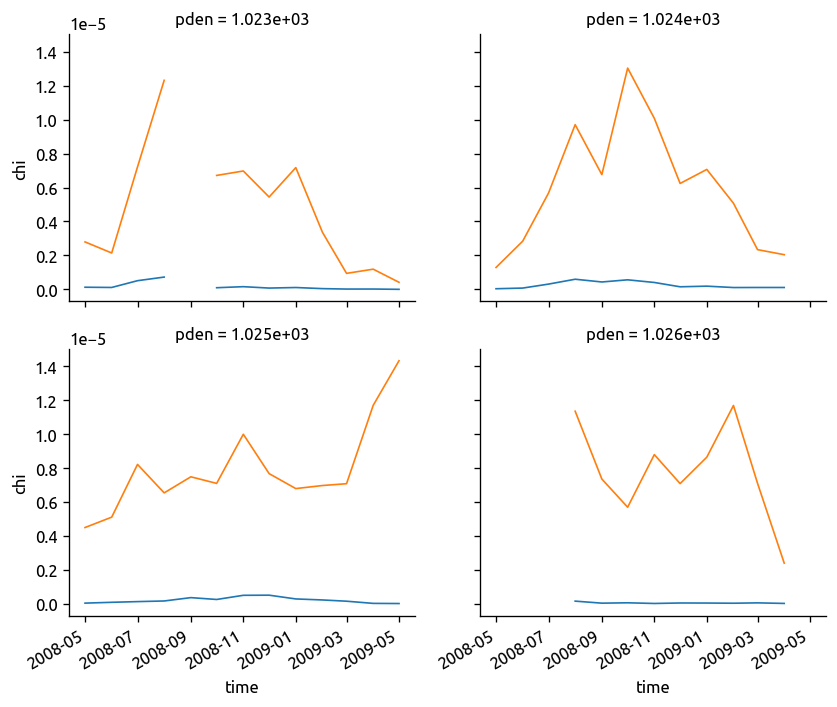
(chidens["chi"] / 2).plot.line(hue="pden")
plt.figure()
(chidens["KtTz"] * isoT["dTdz"]).plot.line(hue="pden")
[<matplotlib.lines.Line2D at 0x7f8787a05450>,
 <matplotlib.lines.Line2D at 0x7f8786e04150>,
 <matplotlib.lines.Line2D at 0x7f8794ec69d0>,
 <matplotlib.lines.Line2D at 0x7f8794ec6990>]
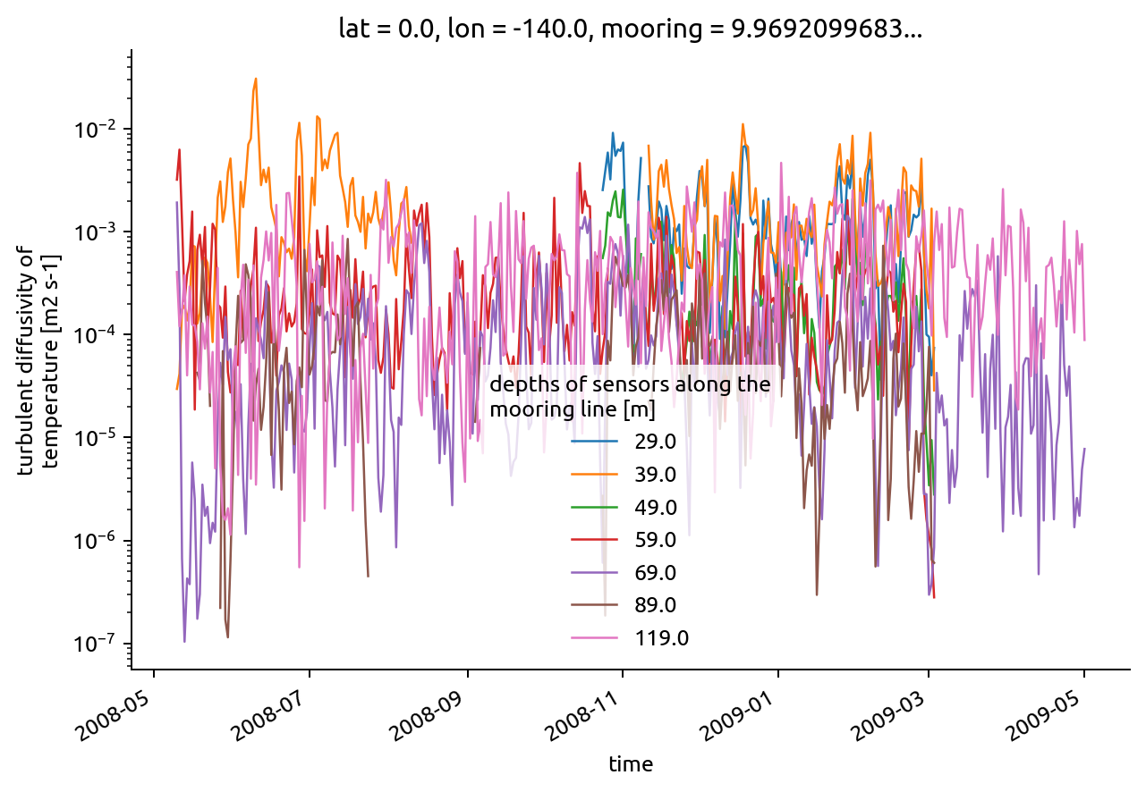
chisub.KT.resample(time="D").mean().plot.line(hue="depth", yscale="log")
[<matplotlib.lines.Line2D at 0x7f38dfaedf10>,
 <matplotlib.lines.Line2D at 0x7f38dfaa3d50>,
 <matplotlib.lines.Line2D at 0x7f38dfb8ce10>,
 <matplotlib.lines.Line2D at 0x7f38e3783a50>,
 <matplotlib.lines.Line2D at 0x7f38e34ce490>,
 <matplotlib.lines.Line2D at 0x7f38dfaba950>,
 <matplotlib.lines.Line2D at 0x7f38dfb84990>]
Testing χ#
eccoT.dTdz.interp(lat=0)
<xarray.DataArray 'dTdz' (pden: 3)>
array([0.03427257, 0.096845  , 0.06992526])
Coordinates:
    lon          float64 220.2
  * pden         (pden) float64 1.024e+03 1.025e+03 1.026e+03
    dz_remapped  (pden) float64 49.35 69.1 35.2
    y            float64 0.0
lat int64 0- pden: 3
- 0.03427 0.09685 0.06993
array([0.03427257, 0.096845 , 0.06992526])
- lon()float64220.2
- units :
- degrees_east
- standard_name :
- longitude
array(220.25)
- pden(pden)float641.024e+03 1.025e+03 1.026e+03
array([1023.525, 1024.675, 1025.75 ])
- dz_remapped(pden)float6449.35 69.1 35.2
array([49.34885735, 69.1025728 , 35.20264963])
- y()float640.0
- description :
- Distance from (0, 220.25)
- units :
- m
- axis :
- Y
array(0.)
- lat()int640
array(0)
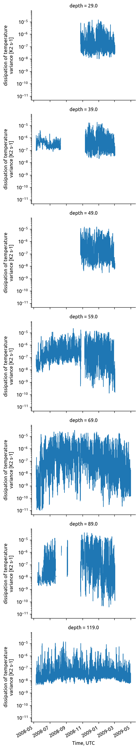
chisub.chi.plot.line(row="depth", yscale="log")
<xarray.plot.facetgrid.FacetGrid at 0x7fd6914463d0>
chi2.dTdz.mean().compute()
<xarray.DataArray 'dTdz' ()>
array(0.03167741)
Coordinates:
    lat      float64 0.0
    lon      float64 -140.0
    mooring  float64 9.969e+36
    chipod   float64 9.969e+36
Attributes:
    long_name:              vertical temperature gradient
    units:                  K m-1
    FillValue:              -9999
    valid_min:              4.9999999999999996e-06
    valid_max:              0.001
    coverage_content_type:  physicalMeasurement
    grid_mapping:           crs
    references:             Moum, J.N. and J.D. Nash, Mixing measurements on ...
    cell_methods:           depth: point, time: mean
    platform:               mooring
instrument: chipod- 0.03168
array(0.03167741)
- lat()float640.0
- long_name :
- latitude
- standard_name :
- latitude
- units :
- degrees_north
- axis :
- Y
- valid_min :
- 0.0
- valid_max :
- 0.0
array(0.)
- lon()float64-140.0
- long_name :
- longitude
- standard_name :
- longitude
- units :
- degrees_east
- axis :
- X
- valid_min :
- -140.0
- valid_max :
- -140.0
array(-140.)
- mooring()float649.969e+36
- long_name :
- Tropical Atmosphere Ocean (TAO) mooring at 0-140W
- comment :
- Global Tropical Moored Buoy Array maintained by NOAA PMEL (https://www.pmel.noaa.gov/gtmba/)
- ncei_code :
- 33TT
array(9.96920997e+36)
- chipod()float649.969e+36
- long_name :
- chipod
- comment :
- instrument designed by the Ocean Mixing Group at Oregon State University to measure turbulence quantities (http://mixing.coas.oregonstate.edu)
array(9.96920997e+36)
- long_name :
- vertical temperature gradient
- units :
- K m-1
- FillValue :
- -9999
- valid_min :
- 4.9999999999999996e-06
- valid_max :
- 0.001
- coverage_content_type :
- physicalMeasurement
- grid_mapping :
- crs
- references :
- Moum, J.N. and J.D. Nash, Mixing measurements on an equatorial ocean mooring, J. Atmos. and Oceanic Tech., 26, 317-336, 2009. pdf: http://mixing.coas.oregonstate.edu/papers/mixing_measurements.pdf
- cell_methods :
- depth: point, time: mean
- platform :
- mooring
- instrument :
- chipod
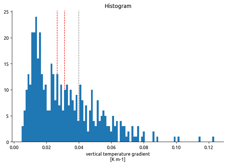
chi2.dTdz.plot.hist(bins=100)
dcpy.plots.linex(0.04)
dcpy.plots.linex(chi2.dTdz.mean(), color="r")
dcpy.plots.linex(chi2.dTdz.compute().median(), color="r")
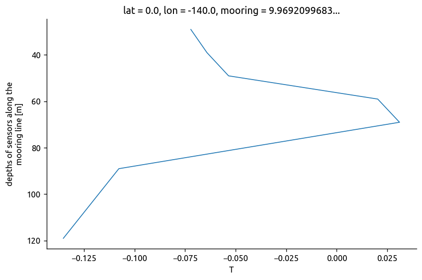
chisub.T.mean("time").differentiate("depth").plot(y="depth", yincrease=False)
[<matplotlib.lines.Line2D at 0x7fd68e34d850>]
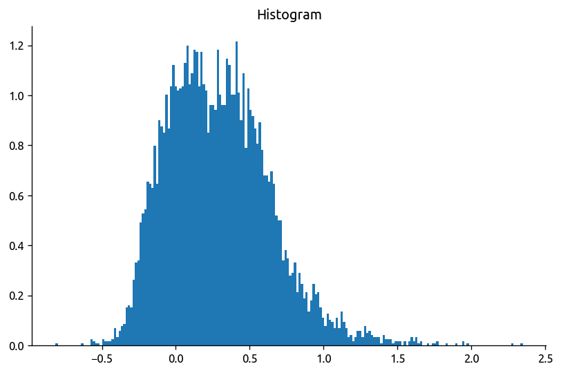
use observed mean dTdz instead of cliamtological mean
meanTz = 0.04
chi2 = (
    chisub.sel(depth=slice(50)).where(chisub.KT < 1e-3).where(chisub.dTdz > 1e-2)
)  # .resample(time="D").mean()
# chi2 = chi2.resample(time="D").mean()

np.log10((chi2.KtTz * meanTz) / (chi2.chi / 2)).plot.hist(bins=200, density=True);
# np.log10((chi2.KtTz * meanTz) / (chi2.chi)).plot.hist(bins=200, density=True);
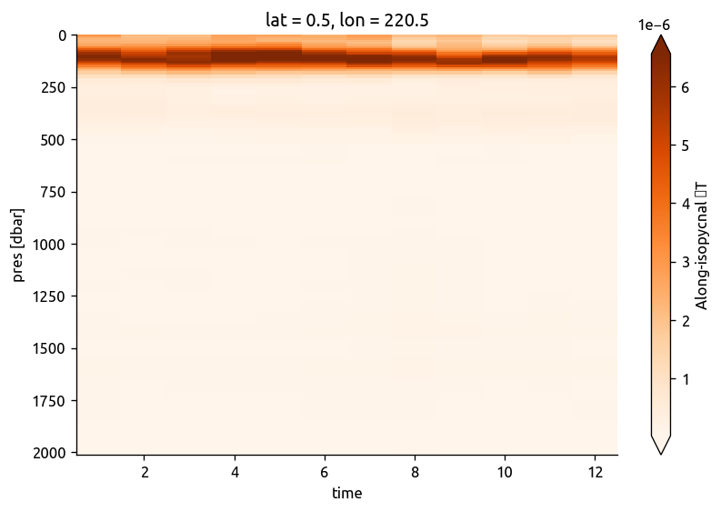
Old stuff#
eccograd, argograd, cole, aber = ed.read_all_datasets(kind="monthly")
argograd.time.attrs["axis"] = "T"
argograd.pres.attrs["positive"] = "down"
argograd.sel(lat=0, lon=360 - 140, method="nearest").dTiso.cf.plot.pcolormesh(
    y="Z", robust=True, cmap=mpl.cm.Oranges
)
<matplotlib.collections.QuadMesh at 0x7fd6930df290>
/home/deepak/miniconda3/envs/dcpy/lib/python3.7/site-packages/matplotlib/backends/backend_agg.py:214: RuntimeWarning: Glyph 8711 missing from current font.
  font.set_text(s, 0.0, flags=flags)
/home/deepak/miniconda3/envs/dcpy/lib/python3.7/site-packages/matplotlib/backends/backend_agg.py:183: RuntimeWarning: Glyph 8711 missing from current font.
  font.set_text(s, 0, flags=flags)
chidens = binned.to_xarray()
grad, _ = ed.bin_to_density_space(
    argograd.sel(lat=0, lon=360 - 140, method="nearest").rename({"ρmean": "rho"}),
    bins=bins,
)
grad = grad.sel(time=chidens.time.dt.month.values).assign_coords(time=chidens.time)
grad
<xarray.Dataset>
Dimensions:   (rho: 4, time: 358)
Coordinates:
  * time      (time) datetime64[ns] 2008-05-10 2008-05-11 ... 2009-05-02
  * rho       (rho) float32 1022.75 1023.25 1024.5 1025.75
    lat       float32 0.5
    lon       float32 220.5
Data variables:
    pres      (time, rho) float64 15.62 50.0 95.0 140.0 ... 50.0 95.0 140.0
    Smean     (time, rho) float32 35.150955 35.16125 ... 35.08096 34.97392
    Tmean     (time, rho) float32 26.652958 25.90761 ... 21.142931 15.874863
    dSdia     (time, rho) float64 0.0004355 0.0007541 ... 0.002183 0.002707
    dSdz      (time, rho) float32 -0.00043551126 0.0005791346 ... 0.002706909
    dSiso     (time, rho) float64 1.038e-06 1.437e-06 ... 2.434e-06 1.457e-06
    dTdia     (time, rho) float64 0.009585 0.0497 0.127 ... 0.0497 0.127 0.08775
    dTdz      (time, rho) float32 0.009585428 0.04970134 ... 0.08775275
    dTiso     (time, rho) float64 2.479e-06 3.539e-06 ... 6.849e-06 5.099e-06
mean_rho (time, rho) float32 1022.9419 1023.1831 ... 1024.4943 1025.7537- rho: 4
- time: 358
- time(time)datetime64[ns]2008-05-10 ... 2009-05-02
array(['2008-05-10T00:00:00.000000000', '2008-05-11T00:00:00.000000000', '2008-05-12T00:00:00.000000000', ..., '2009-04-30T00:00:00.000000000', '2009-05-01T00:00:00.000000000', '2009-05-02T00:00:00.000000000'], dtype='datetime64[ns]') - rho(rho)float321022.75 1023.25 1024.5 1025.75
- positive :
- down
array([1022.75, 1023.25, 1024.5 , 1025.75], dtype=float32)
- lat()float320.5
- axis :
- Y
- point_spacing :
- even
- units :
- degrees_north
array(0.5, dtype=float32)
- lon()float32220.5
- axis :
- X
- modulo :
- 360.0
- point_spacing :
- even
- units :
- degrees_east
array(220.5, dtype=float32)
- pres(time, rho)float6415.62 50.0 95.0 ... 50.0 95.0 140.0
array([[ 15.625, 50. , 95. , 140. ], [ 15.625, 50. , 95. , 140. ], [ 15.625, 50. , 95. , 140. ], ..., [ 15.625, 50. , 95. , 140. ], [ 15.625, 50. , 95. , 140. ], [ 15.625, 50. , 95. , 140. ]]) - Smean(time, rho)float3235.150955 35.16125 ... 34.97392
array([[35.150955, 35.16125 , 35.08096 , 34.97392 ], [35.150955, 35.16125 , 35.08096 , 34.97392 ], [35.150955, 35.16125 , 35.08096 , 34.97392 ], ..., [35.172356, 35.171585, 35.101944, 34.97047 ], [35.150955, 35.16125 , 35.08096 , 34.97392 ], [35.150955, 35.16125 , 35.08096 , 34.97392 ]], dtype=float32) - Tmean(time, rho)float3226.652958 25.90761 ... 15.874863
array([[26.652958, 25.90761 , 21.142931, 15.874863], [26.652958, 25.90761 , 21.142931, 15.874863], [26.652958, 25.90761 , 21.142931, 15.874863], ..., [26.782187, 25.793835, 21.372473, 15.860222], [26.652958, 25.90761 , 21.142931, 15.874863], [26.652958, 25.90761 , 21.142931, 15.874863]], dtype=float32) - dSdia(time, rho)float640.0004355 0.0007541 ... 0.002707
array([[0.00043551, 0.0007541 , 0.00218337, 0.00270691], [0.00043551, 0.0007541 , 0.00218337, 0.00270691], [0.00043551, 0.0007541 , 0.00218337, 0.00270691], ..., [0.00014337, 0.0005291 , 0.00237643, 0.00276388], [0.00043551, 0.0007541 , 0.00218337, 0.00270691], [0.00043551, 0.0007541 , 0.00218337, 0.00270691]]) - dSdz(time, rho)float32-0.00043551126 ... 0.002706909
array([[-4.3551126e-04, 5.7913462e-04, 2.1833738e-03, 2.7069091e-03], [-4.3551126e-04, 5.7913462e-04, 2.1833738e-03, 2.7069091e-03], [-4.3551126e-04, 5.7913462e-04, 2.1833738e-03, 2.7069091e-03], ..., [ 7.6707205e-05, 3.9863586e-04, 2.3764293e-03, 2.7638753e-03], [-4.3551126e-04, 5.7913462e-04, 2.1833738e-03, 2.7069091e-03], [-4.3551126e-04, 5.7913462e-04, 2.1833738e-03, 2.7069091e-03]], dtype=float32) - dSiso(time, rho)float641.038e-06 1.437e-06 ... 1.457e-06
array([[1.03800666e-06, 1.43683528e-06, 2.43359509e-06, 1.45745652e-06], [1.03800666e-06, 1.43683528e-06, 2.43359509e-06, 1.45745652e-06], [1.03800666e-06, 1.43683528e-06, 2.43359509e-06, 1.45745652e-06], ..., [1.12516232e-06, 1.38026710e-06, 2.37830918e-06, 1.52299625e-06], [1.03800666e-06, 1.43683528e-06, 2.43359509e-06, 1.45745652e-06], [1.03800666e-06, 1.43683528e-06, 2.43359509e-06, 1.45745652e-06]]) - dTdia(time, rho)float640.009585 0.0497 ... 0.127 0.08775
array([[0.00958543, 0.04970134, 0.1269882 , 0.08775276], [0.00958543, 0.04970134, 0.1269882 , 0.08775276], [0.00958543, 0.04970134, 0.1269882 , 0.08775276], ..., [0.01437708, 0.05530132, 0.12062849, 0.09751533], [0.00958543, 0.04970134, 0.1269882 , 0.08775276], [0.00958543, 0.04970134, 0.1269882 , 0.08775276]]) - dTdz(time, rho)float320.009585428 ... 0.08775275
array([[0.00958543, 0.04970134, 0.1269882 , 0.08775275], [0.00958543, 0.04970134, 0.1269882 , 0.08775275], [0.00958543, 0.04970134, 0.1269882 , 0.08775275], ..., [0.01437709, 0.05530132, 0.12062848, 0.09751533], [0.00958543, 0.04970134, 0.1269882 , 0.08775275], [0.00958543, 0.04970134, 0.1269882 , 0.08775275]], dtype=float32) - dTiso(time, rho)float642.479e-06 3.539e-06 ... 5.099e-06
array([[2.47936121e-06, 3.53900669e-06, 6.84937495e-06, 5.09938519e-06], [2.47936121e-06, 3.53900669e-06, 6.84937495e-06, 5.09938519e-06], [2.47936121e-06, 3.53900669e-06, 6.84937495e-06, 5.09938519e-06], ..., [2.68430569e-06, 3.40710693e-06, 6.68691848e-06, 5.39222018e-06], [2.47936121e-06, 3.53900669e-06, 6.84937495e-06, 5.09938519e-06], [2.47936121e-06, 3.53900669e-06, 6.84937495e-06, 5.09938519e-06]]) - mean_rho(time, rho)float321022.9419 1023.1831 ... 1025.7537
array([[1022.9419 , 1023.1831 , 1024.4943 , 1025.7537 ],
       [1022.9419 , 1023.1831 , 1024.4943 , 1025.7537 ],
       [1022.9419 , 1023.1831 , 1024.4943 , 1025.7537 ],
       ...,
       [1022.91693, 1023.2262 , 1024.4518 , 1025.7538 ],
       [1022.9419 , 1023.1831 , 1024.4943 , 1025.7537 ],
       [1022.9419 , 1023.1831 , 1024.4943 , 1025.7537 ]], dtype=float32)
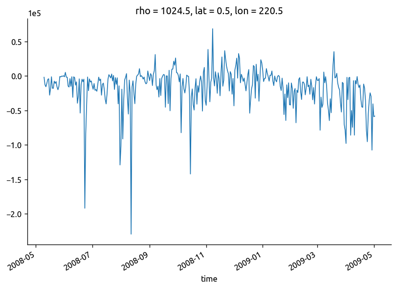
chidens["rho"] = grad["rho"]
Ke = (chidens["chi"] / 2 - np.abs(chidens["KtTz"] * grad["dTdz"] / 3)) / (
    grad["dTiso"] ** 2
)
Ke
<xarray.DataArray (rho: 4, time: 358)>
array([[            nan,             nan,             nan, ...,
                    nan,             nan,             nan],
       [ 11726.46725949,   8248.95985651,   5027.56820076, ...,
          -204.25370459,   -334.24473111,   -187.44859464],
       [ -1879.12790238, -12763.75317847, -15621.72404617, ...,
        -40449.6307827 , -59050.73202118, -58244.54230018],
       [            nan,             nan,             nan, ...,
                    nan,             nan,             nan]])
Coordinates:
  * rho      (rho) float32 1022.75 1023.25 1024.5 1025.75
  * time     (time) datetime64[ns] 2008-05-10 2008-05-11 ... 2009-05-02
    lat      float32 0.5
lon float32 220.5- rho: 4
- time: 358
- nan nan nan nan nan nan nan nan ... nan nan nan nan nan nan nan nan
array([[ nan, nan, nan, ..., nan, nan, nan], [ 11726.46725949, 8248.95985651, 5027.56820076, ..., -204.25370459, -334.24473111, -187.44859464], [ -1879.12790238, -12763.75317847, -15621.72404617, ..., -40449.6307827 , -59050.73202118, -58244.54230018], [ nan, nan, nan, ..., nan, nan, nan]]) - rho(rho)float321022.75 1023.25 1024.5 1025.75
- positive :
- down
array([1022.75, 1023.25, 1024.5 , 1025.75], dtype=float32)
- time(time)datetime64[ns]2008-05-10 ... 2009-05-02
array(['2008-05-10T00:00:00.000000000', '2008-05-11T00:00:00.000000000', '2008-05-12T00:00:00.000000000', ..., '2009-04-30T00:00:00.000000000', '2009-05-01T00:00:00.000000000', '2009-05-02T00:00:00.000000000'], dtype='datetime64[ns]') - lat()float320.5
- axis :
- Y
- point_spacing :
- even
- units :
- degrees_north
array(0.5, dtype=float32)
- lon()float32220.5
- axis :
- X
- modulo :
- 360.0
- point_spacing :
- even
- units :
- degrees_east
array(220.5, dtype=float32)
Ke.isel(rho=2).plot()
[<matplotlib.lines.Line2D at 0x7feb1dc04650>]
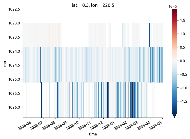
(chidens["chi"] / 2 - np.abs(chidens["KtTz"] * grad["dTdz"])).cf.plot(
    x="time", y="rho", robust=True
)
<matplotlib.collections.QuadMesh at 0x7feb1c082110>