T-S diagrams from TAO & Argo at (0, 145W→135W)

In this notebook 140W really means (145W → 135W)

looking at TS diagrams across latitudes.

1. During TIW activity do we see more stirring near the equator or off the equator?

2. If salinity is a minor contributor to density, do we really expect to see T-S scatter as a signal of eddy stirring?

(Surprising conclusions)

1. T-S spread is similar in all ENSO phases. There is some separation in temperature (as expected)

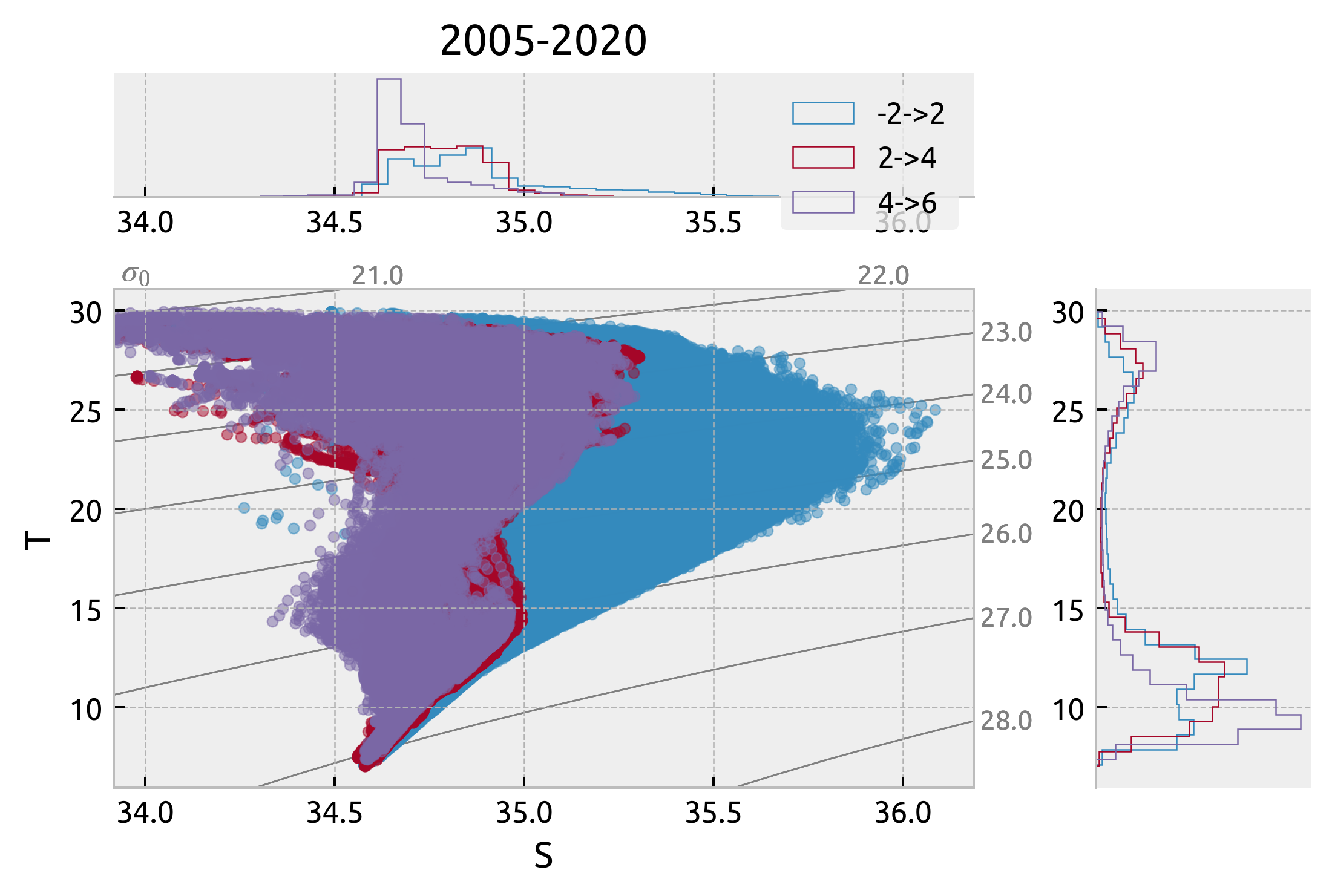
2. Latitudinal variation in T-S spread is big; but again ENSO variation is minimal at all latitudes I’ve checked.

%load_ext watermark

import cf_xarray
import dcpy
import distributed
import matplotlib as mpl
import matplotlib.pyplot as plt
import numpy as np
import pandas as pd
import pump
import xfilter
import xgcm
import xhistogram

import eddydiff as ed
import xarray as xr

xr.set_options(keep_attrs=True)

%watermark -iv
plt.rcParams["figure.dpi"] = 180
plt.rcParams["savefig.dpi"] = 200

plt.style.use("bmh")

numpy      : 1.20.2
xarray     : 0.17.1.dev3+g48378c4b1
xfilter    : 0.1.dev41+geb0277f
dcpy       : 0.1
cf_xarray  : 0.4.1.dev21+gab9dc66
matplotlib : 3.4.1
xgcm       : 0.5.1
eddydiff   : 0.1
pump       : 0.1
xhistogram : 0.1.3+37.g7b706e8
pandas     : 1.2.3
distributed: 2021.4.0

if "client" in locals():
    client.close()
client = distributed.Client(n_workers=3, processes=False, memory_limit="8GB")
client

TIWKE from TAO

tao = xr.open_zarr(
    "/home/deepak/work/pump/notebooks/tao_eq_hr_gridded.zarr/", consolidated=True
).sel(longitude=-140, time=slice("1996", None))

vmean = (
    tao.v.sel(depth=slice(-80, 0))
    .mean("depth")
    .chunk({"time": -1})
    .interpolate_na("time", max_gap="10D")
    .compute()
)

# Moum et al. 2009 metric
v = xfilter.bandpass(
    vmean,
    "time",
    freq=[1 / 12, 1 / 33],
    cycles_per="D",
    debug=False,
    num_discard=120,
)
tiwke = xfilter.lowpass(
    v**2 / 2,
    "time",
    freq=1 / 20,
    cycles_per="D",
)
tiwke.attrs = {"long_name": "TIW KE", "units": "m²/s²"}
tiwke = tiwke

/home/deepak/miniconda3/envs/dcpy/lib/python3.8/site-packages/dask/array/numpy_compat.py:39: RuntimeWarning: invalid value encountered in true_divide
  x = np.divide(x1, x2, out)

Argo

Read data

ds = xr.load_dataset("../datasets/argo/tao.nc")
ds.coords["year"] = ds.TIME.dt.year
ds

<xarray.Dataset>
Dimensions:                (N_POINTS: 1327818)
Coordinates:
    LATITUDE               (N_POINTS) float64 6.221 6.221 ... -1.509 -1.509
    LONGITUDE              (N_POINTS) float64 -140.0 -140.0 ... -138.7 -138.7
    TIME                   (N_POINTS) datetime64[ns] 2005-03-08T17:40:05 ... ...
    year                   (N_POINTS) int64 2005 2005 2005 ... 2020 2020 2020
Dimensions without coordinates: N_POINTS
Data variables: (12/13)
    CONFIG_MISSION_NUMBER  (N_POINTS) int64 1 1 1 1 1 1 1 ... 84 84 84 84 84 84
    CYCLE_NUMBER           (N_POINTS) int64 1 1 1 1 1 1 1 ... 84 84 84 84 84 84
    DATA_MODE              (N_POINTS) object 'D' 'D' 'D' 'D' ... 'A' 'A' 'A' 'A'
    DIRECTION              (N_POINTS) object 'A' 'A' 'A' 'A' ... 'A' 'A' 'A' 'A'
    PLATFORM_NUMBER        (N_POINTS) int64 5900884 5900884 ... 1902197 1902197
    POSITION_QC            (N_POINTS) int64 1 1 1 1 1 1 1 1 ... 1 1 1 1 1 1 1 1
    ...                     ...
    PRES_QC                (N_POINTS) int64 1 1 1 1 1 1 1 1 ... 1 1 1 1 1 1 1 1
    PSAL                   (N_POINTS) float64 34.85 34.85 34.85 ... 34.62 34.62
    PSAL_QC                (N_POINTS) int64 1 1 1 1 1 1 1 1 ... 1 1 1 1 1 1 1 1
    TEMP                   (N_POINTS) float64 27.97 27.97 27.97 ... 7.57 7.555
    TEMP_QC                (N_POINTS) int64 1 1 1 1 1 1 1 1 ... 1 1 1 1 1 1 1 1
    TIME_QC                (N_POINTS) int64 1 1 1 1 1 1 1 1 ... 1 1 1 1 1 1 1 1
Attributes:
    DATA_ID:              ARGO
    DOI:                  http://doi.org/10.17882/42182
    Fetched_from:         https://www.ifremer.fr/erddap
    Fetched_by:           deepak
    Fetched_date:         2021/04/08
    Fetched_constraints:  [x=-145.00/-135.00; y=-2.00/8.00; z=0.0/500.0; t=20...
    Fetched_uri:          https://www.ifremer.fr/erddap/tabledap/ArgoFloats.n...
    history:              Variables filtered according to DATA_MODE; Variable...

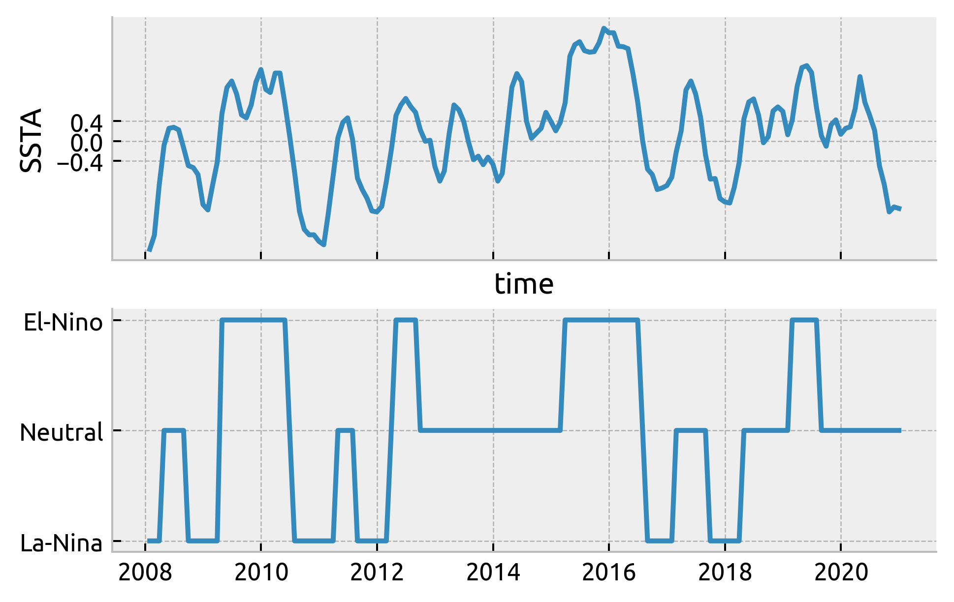
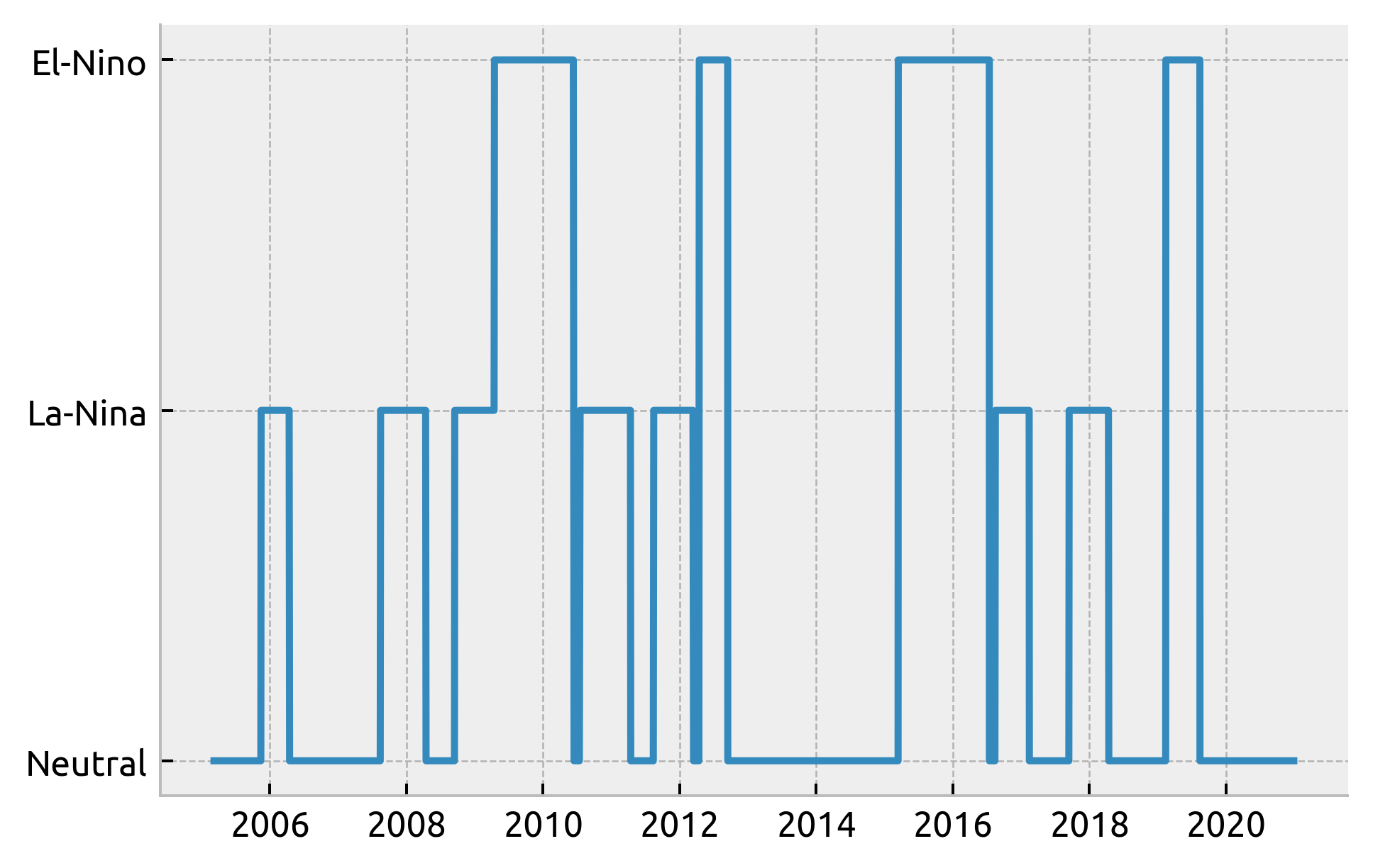
Generate ENSO labels

From Anna; Some Trenberth metric

1. Use NINO34 SST annomaly (w.r.t mean from 18xx)

2. At least 6 month long periods of SSTA > 0.4 (El-nino) & SSTA < -0.4 (La-Nina). Neutral everywhere else

from dcpy.util import block_lengths

from xarray.core.missing import _get_nan_block_lengths, get_clean_interp_index

nino34 = pump.obs.process_nino34()
ssta = nino34 - nino34.mean()  # .rolling(time=6, center=True).mean()

enso = xr.full_like(ssta, fill_value="Neutral", dtype="U8")
index = ssta.indexes["time"] - ssta.indexes["time"][0]
en_mask = _get_nan_block_lengths(
    xr.where(ssta > 0.4, np.nan, 0), dim="time", index=index
) >= pd.Timedelta("169d")
ln_mask = _get_nan_block_lengths(
    xr.where(ssta < -0.4, np.nan, 0), dim="time", index=index
) >= pd.Timedelta("169d")
# neut_mask = _get_nan_block_lengths(xr.where((ssta < 0.5) & (ssta > -0.5), np.nan, 0), dim="time", index=index) >= pd.Timedelta("120d")

enso.loc[en_mask] = "El-Nino"
enso.loc[ln_mask] = "La-Nina"
# enso.loc[neut_mask] = "Neutral"

enso.name = "enso_phase"
enso.attrs[
    "description"
] = "ENSO phase; El-Nino = NINO34 SSTA > 0.4 for at least 6 months; La-Nina = NINO34 SSTA < -0.4 for at least 6 months"
enso

<xarray.DataArray 'enso_phase' (time: 1812)>
array(['Neutral', 'Neutral', 'Neutral', ..., 'Neutral', 'Neutral',
       'Neutral'], dtype='<U8')
Coordinates:
  * time     (time) datetime64[ns] 1870-01-31 1870-02-28 ... 2020-12-31
Attributes:
    description:  ENSO phase; El-Nino = NINO34 SSTA > 0.4 for at least 6 mont...

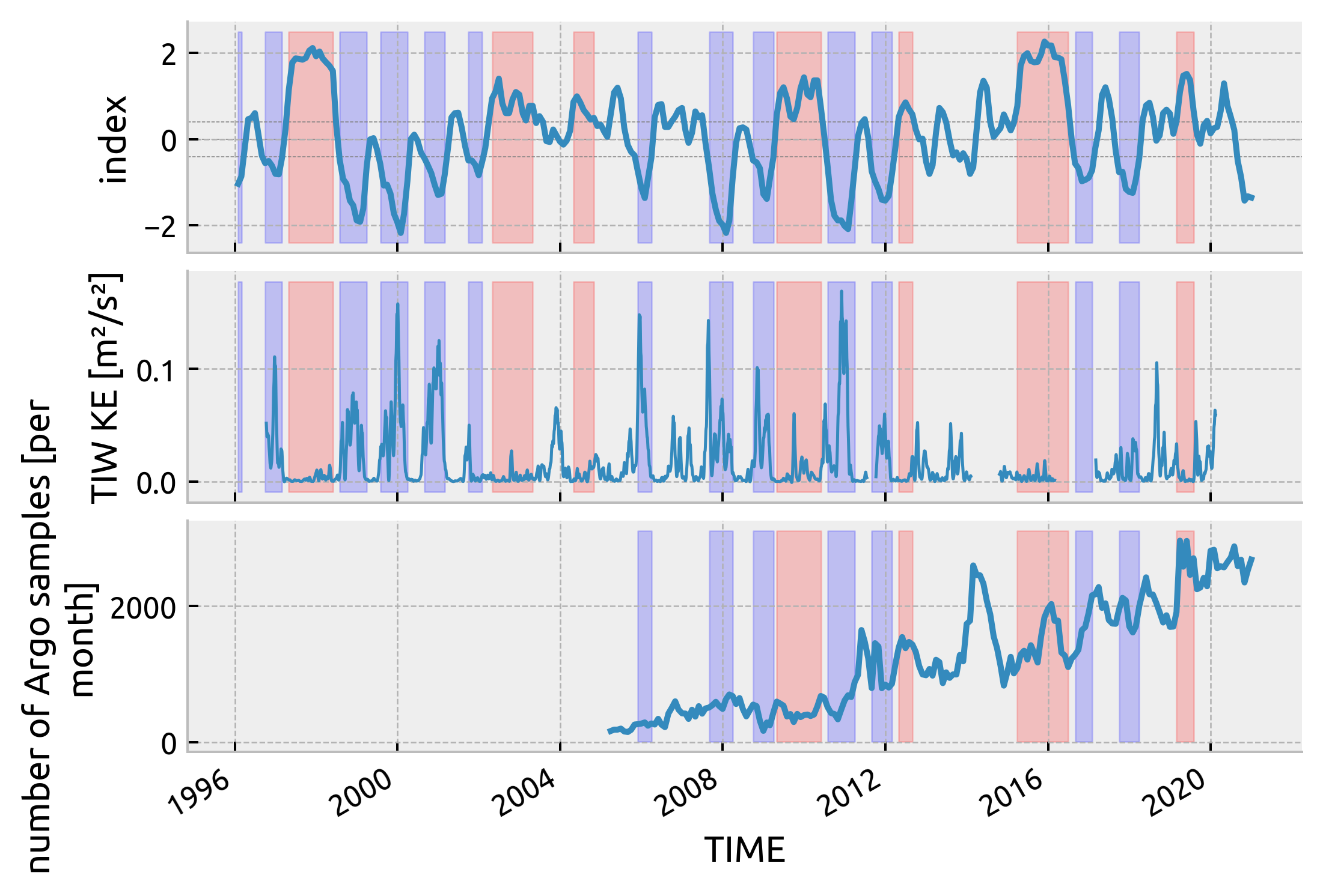
Test against TIWKE

counts = (
    ds.query({"N_POINTS": "PRES > 35 and PRES < 120"})
    .TEMP.swap_dims({"N_POINTS": "TIME"})
    .resample(TIME="M")
    .count()
)
counts.attrs = {"long_name": "number of Argo samples", "units": "per month"}

from pump.plots import highlight_enso

ssta_ = dcpy.util.slice_like(ssta, tiwke)
enso_ = dcpy.util.slice_like(enso, tiwke)

f, axx = plt.subplots(3, 1, sharex=True, constrained_layout=True)
ssta_.plot(x="time", ax=axx[0])
highlight_enso(axx[0], enso_)
dcpy.plots.liney([-0.4, 0, 0.4], ax=axx[0], lw=0.3)

tiwke.plot(ax=axx[1], lw=1)
highlight_enso(axx[1], enso_)

counts.plot(ax=axx[2])
highlight_enso(axx[2], enso_.sel(time=slice("2005", None)))

dcpy.plots.clean_axes(np.atleast_2d(axx).T)

check ENSO phase calculation

f, ax = plt.subplots(2, 1, sharex=True)
(nino34 - nino34.mean()).sel(time=slice("2008", None)).plot(ax=ax[0])
ax[0].set_ylabel("SSTA")
ax[0].set_yticks([-0.4, 0, 0.4])
plt.plot(enso.time.sel(time=slice("2008", None)), enso.sel(time=slice("2008", None)))

[<matplotlib.lines.Line2D at 0x7fd20a9eac70>]

ds.coords["enso_phase"] = enso.sel(time=ds.TIME, method="nearest")
plt.plot(ds.TIME, ds.enso_phase)

[<matplotlib.lines.Line2D at 0x7fd4c8612d60>]

Latitudinal variation at 140W

subset = ds.query({"N_POINTS": "LATITUDE > -2 & LATITUDE < 2"})
_, ax = dcpy.oceans.TSplot(subset.PSAL, subset.TEMP, hexbin=False)

subset = ds.query({"N_POINTS": "LATITUDE > 2 & LATITUDE < 4"})
dcpy.oceans.TSplot(subset.PSAL, subset.TEMP, hexbin=False, ax=ax)

subset = ds.query({"N_POINTS": "LATITUDE > 4 & LATITUDE < 6"})
dcpy.oceans.TSplot(subset.PSAL, subset.TEMP, hexbin=False, ax=ax)

ax["s"].legend(["-2->2", "2->4", "4->6"])
ax["s"].set_title("2005-2020")

Text(0.5, 1.0, '2005-2020')

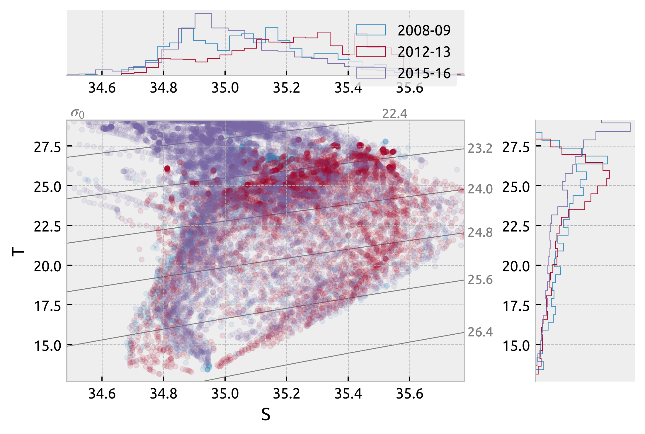
Interannual variation at (2S→2N, -140)

Picked out two La-Nina(2008, 09; 2012, 13) and one El-Nino period (2015, 2016). They look very similar

kwargs = dict(kind="scatter", plot_kwargs=dict(alpha=0.1))

common = "LONGITUDE > -142 & LONGITUDE < -138 & LATITUDE > -2 & LATITUDE < 2 & PRES > 35 & PRES < 120"
subset = ds.query({"N_POINTS": f"{common} & (year == 2008 | year == 2009)"})
_, ax = dcpy.oceans.TSplot(subset.PSAL, subset.TEMP, **kwargs)

subset = ds.query({"N_POINTS": f"{common} & (year == 2012 | year == 2013)"})
dcpy.oceans.TSplot(subset.PSAL, subset.TEMP, **kwargs, ax=ax)

subset = ds.query({"N_POINTS": f"{common} & (year == 2015 | year == 2016)"})
dcpy.oceans.TSplot(subset.PSAL, subset.TEMP, **kwargs, ax=ax)

ax["s"].legend(["2008-09", "2012-13", "2015-16"])

<matplotlib.legend.Legend at 0x7fd1eab81970>

distributed.utils_perf - WARNING - full garbage collections took 10% CPU time recently (threshold: 10%)
distributed.utils_perf - WARNING - full garbage collections took 10% CPU time recently (threshold: 10%)

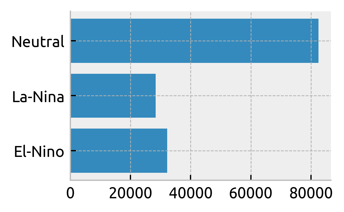
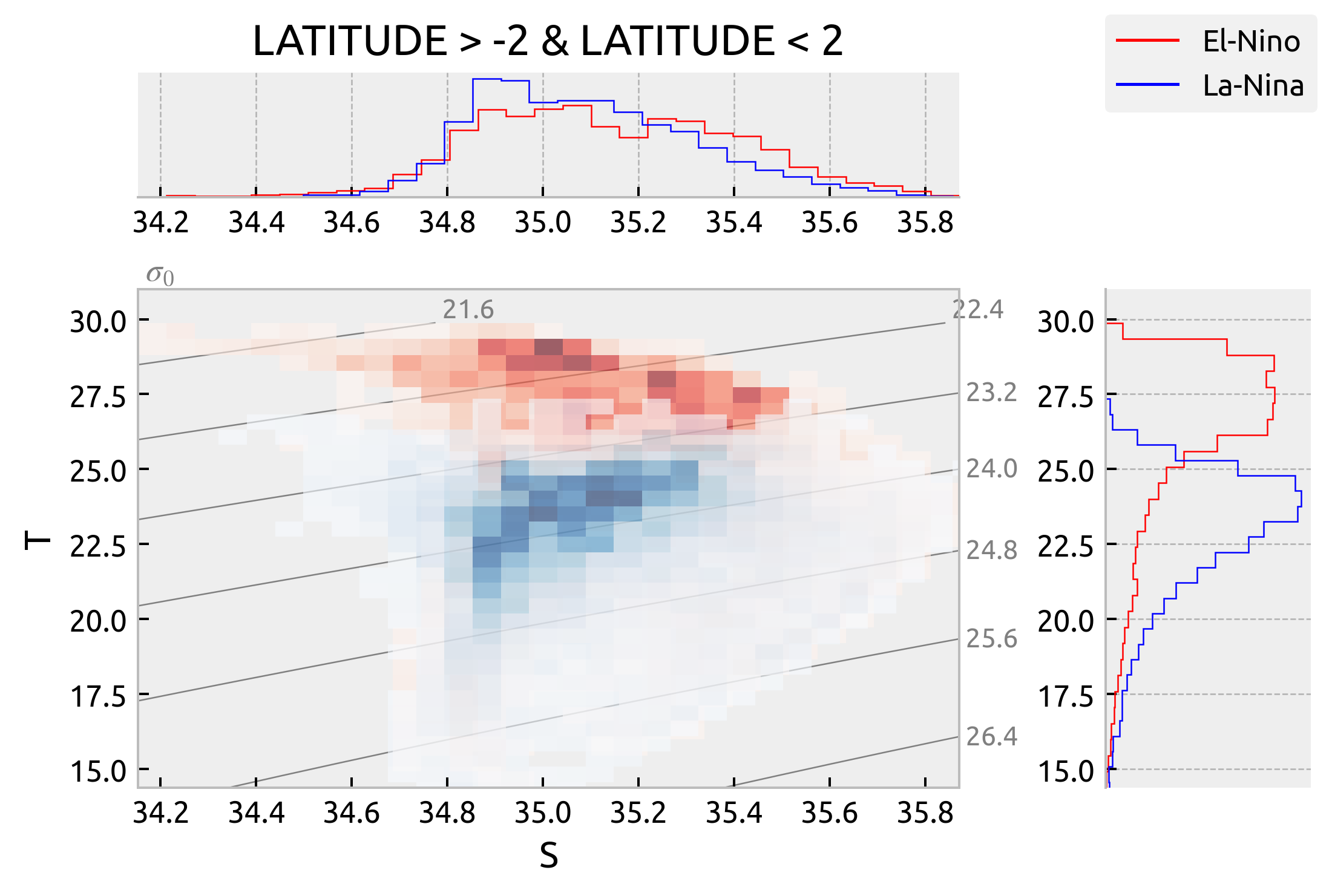
T-S diagram variation with ENSO phase

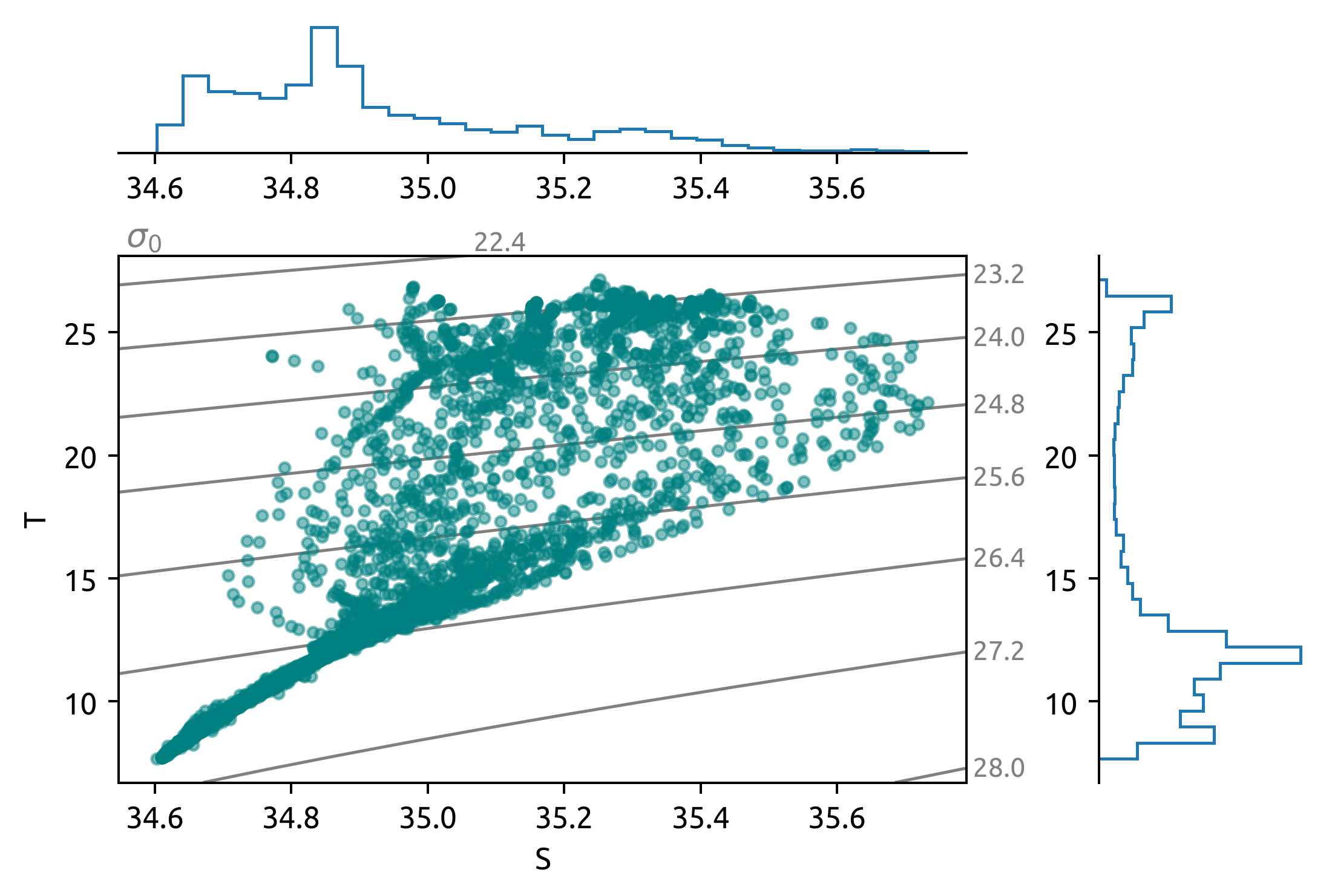
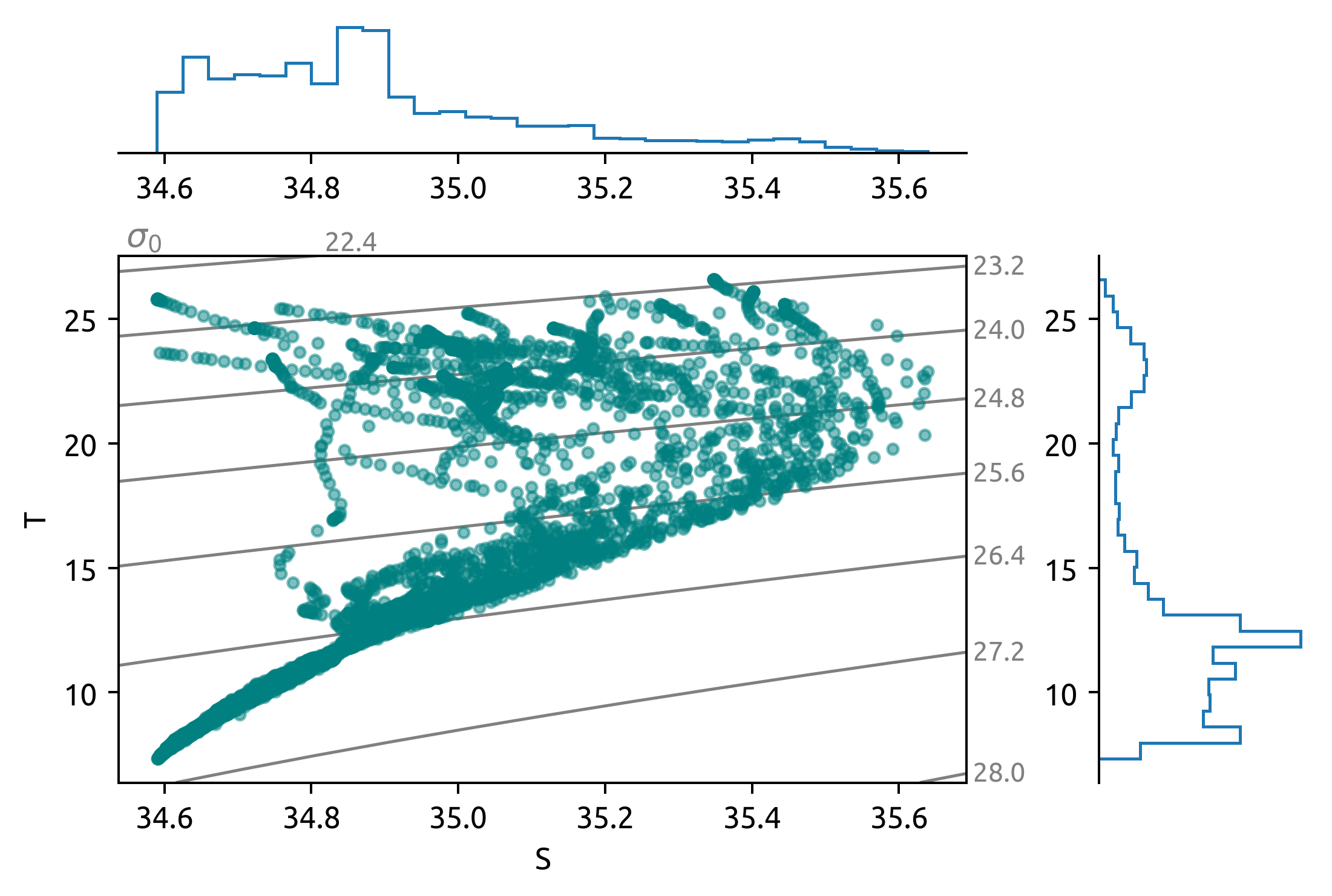
This is a TS diagram of Argo profiles between 135W→145W, 2S→2N; grouped by ENSO phase.

1. El-Nino:

   • isopycnal scatter at warmer isotherms during El-Ninos (top 100m). Where is that coming from.

   • Below ≈ 100m the TS relationship is tight with two end-members? Some of this is a function of spatial extent.

2. La-Nina:

   • Similar scatter to El-Nino which is surprising

3. Neutral:

   • Lots of scatter! But also lots more points.

   • higher salinity water appears

• could add depth contours.

counts = (
    ds.query({"N_POINTS": f"LATITUDE > -2 & LATITUDE < 2 & PRES > 35 & PRES < 120"})
    .groupby("enso_phase")
    .count()
)
plt.barh(counts.enso_phase, counts.TEMP)
plt.gcf().set_size_inches((3, 2))

def plot_TS(latitude_string):
    """Plot a TS diagram per ENSO phase"""
    from matplotlib.lines import Line2D

    kwargs = dict(
        hexbin=True,
        plot_kwargs={"alpha": 0.3, "mincnt": 10, "norm": mpl.colors.LogNorm(1, 100)},
    )
    # kwargs = dict(kind="scatter", plot_kwargs={"alpha": 0.1})
    kwargs = dict(kind="hist", equalize=False, plot_kwargs={"alpha": 0.6})

    ax = None
    labels = []
    lines = []

    for phase, cmap, color in [
        ["El-Nino", mpl.cm.Reds, "red"],
        # ["Neutral", mpl.cm.Greys, "black"],
        ["La-Nina", mpl.cm.Blues, "blue"],
    ]:
        subset = ds.query(
            {
                "N_POINTS": f"{latitude_string} & enso_phase == {phase!r} & PRES > 35 & PRES < 100"
            }
        )
        kwargs["plot_kwargs"]["cmap"] = cmap
        if ax is not None:
            kwargs.update({"label_spines": False, "rho_levels": None})

        hdl, ax = dcpy.oceans.TSplot(
            subset.PSAL, subset.TEMP, color=color, **kwargs, ax=ax
        )
        lines.append(Line2D([0], [0], color=color, lw=1))
        labels.append(phase)

    ax["ts"].set_ylim([None, 31])
    ax["t"].get_figure().legend(handles=lines, labels=labels, loc="upper right")
    ax["s"].set_title(latitude_string)

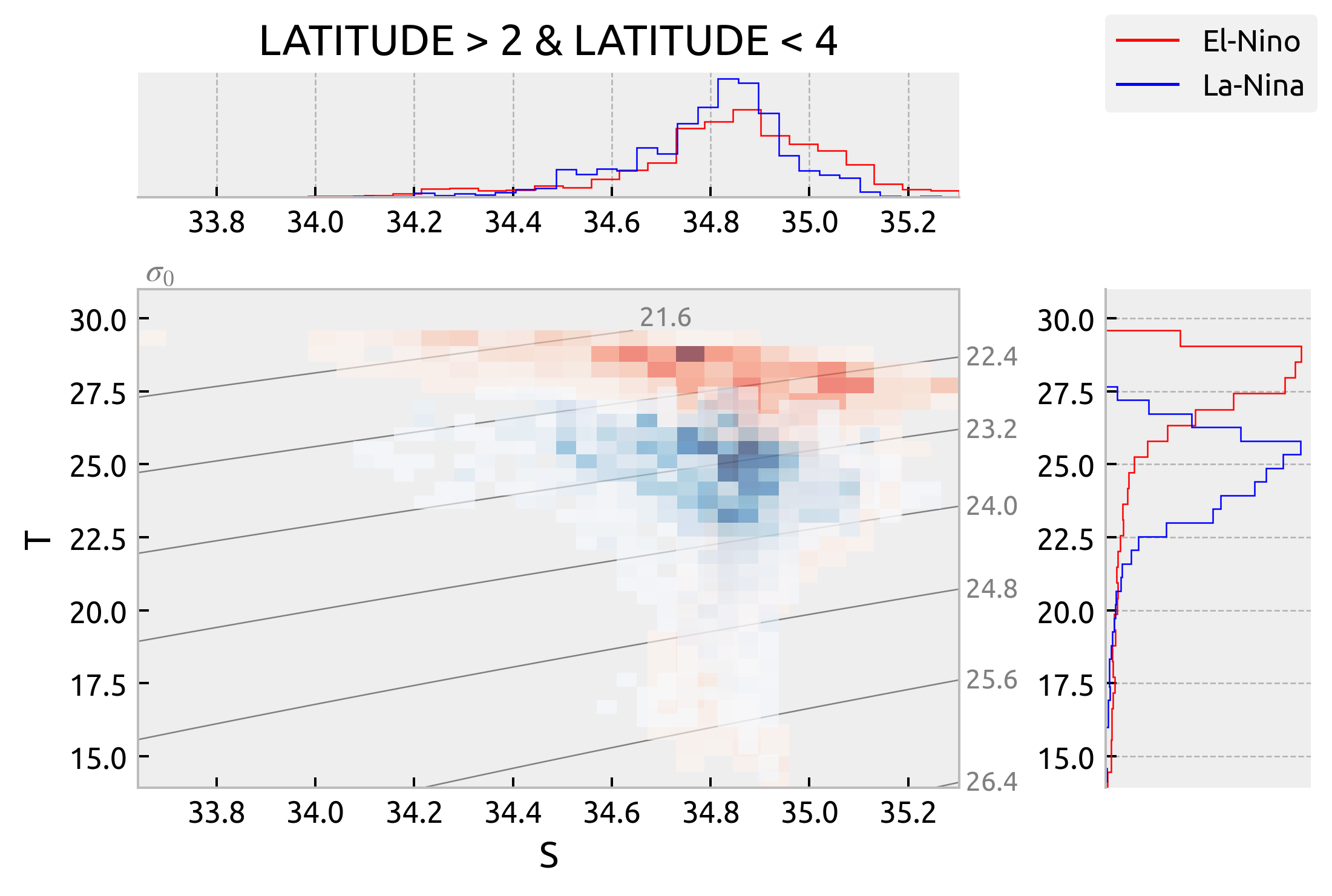
It looks like there is latitudinal variation in T-S spread along isopycnals but not really an ENSO phase variation. The La-Nina and Neutral TS diagrams basically overlap but we can see that the La-Nina and El-Nino diagrams are really only different in that the El-Nino one is warmer. The spread looks the same.

1. plot distributions along 24.5 isopycnal

plot_TS(latitude_string="LATITUDE > -2 & LATITUDE < 2")
plot_TS(latitude_string="LATITUDE > 2 & LATITUDE < 4")

---

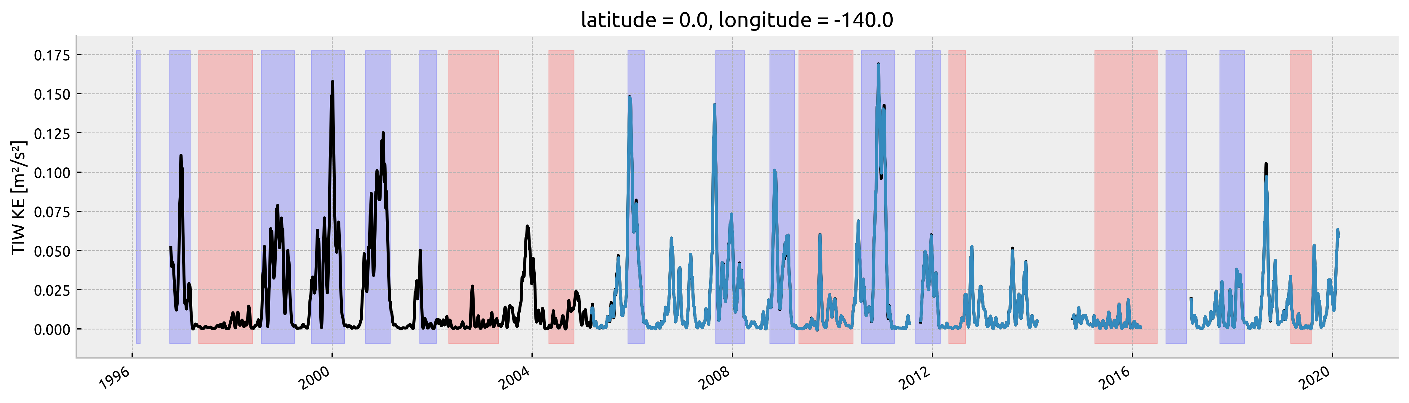
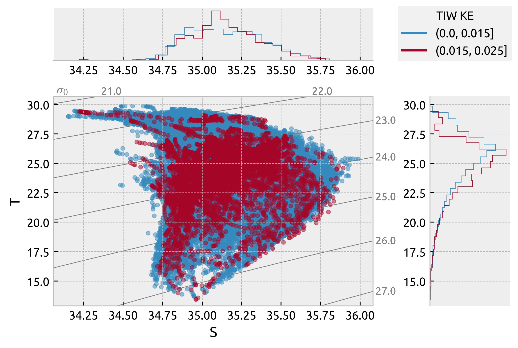
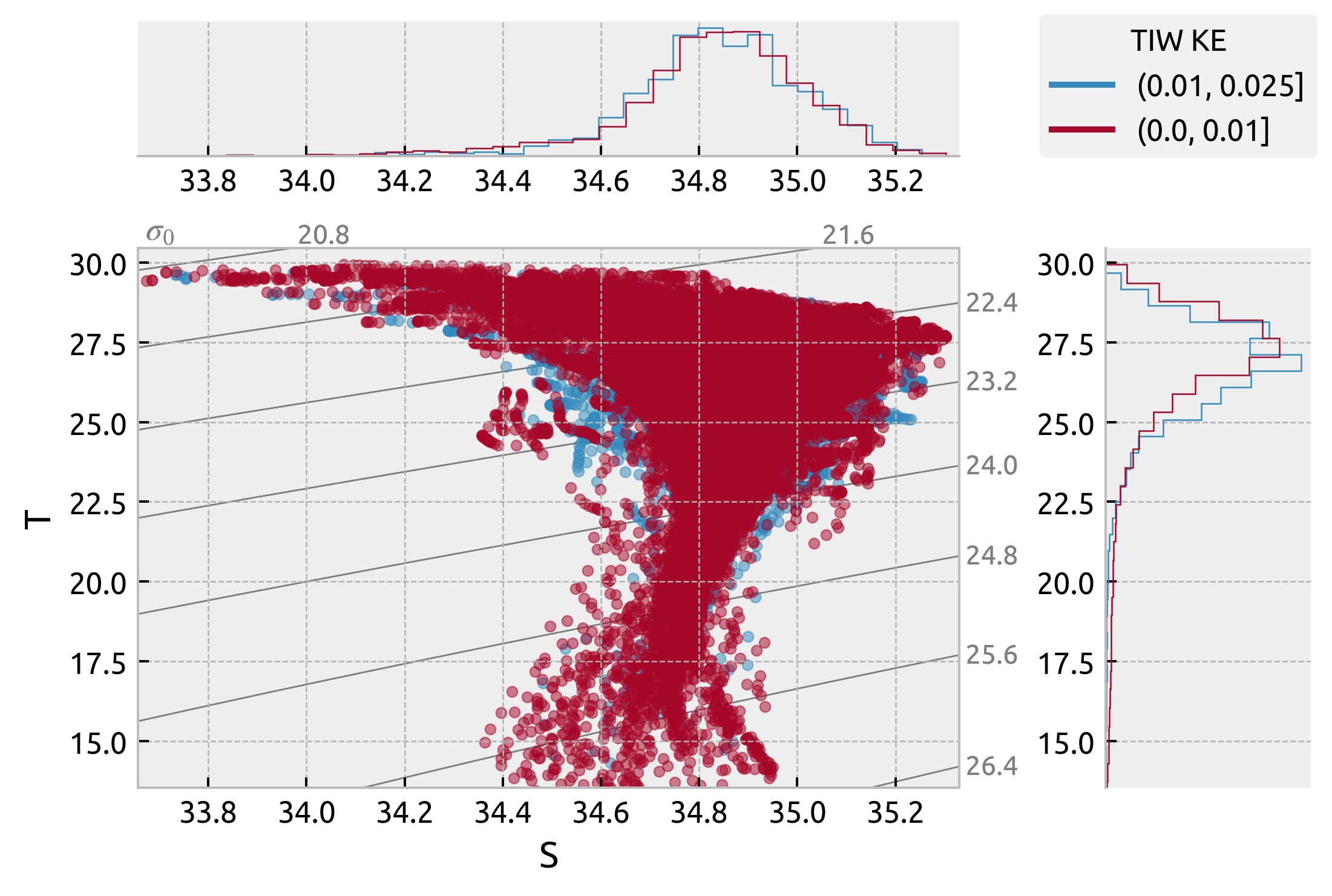
Variation of T-S with TIWKE at (0, 140W)

Looks the same even for weak TIWs.

This won’t really recover the La-Nina/El-Nino plot because you can have periods of weak TIW KE during La-Nina conditions

TODO: I think I might need to set TIWKE for a profile as (mean TIWKE within a 5-10 day window)?

ds["tiwke"] = tiwke.sel(time=ds.TIME, method="pad")

da = tiwke.copy(deep=True)

tiwke.plot(x="time", color="k", size=4, aspect=4)
ds.tiwke.plot(x="TIME")
highlight_enso(ax=plt.gca(), enso=enso.sel(time=slice("1996", None)))
plt.gca().set_xlabel("")

Text(0.5, 0, '')

tiwkegrouped = ds.groupby_bins("tiwke", bins=[0, 0.015, 0.025])

from matplotlib.lines import Line2D

ax = None
labels = []
lines = []
for label, group in tiwkegrouped:
    group = group.query(
        {"N_POINTS": "LATITUDE > -2 & LATITUDE < 2 & PRES > 35 & PRES < 100"}
    )
    hdl, axxx = dcpy.oceans.TSplot(group.PSAL, group.TEMP, kind="scatter", ax=ax)
    if ax is None:
        ax = axxx
    lines.append(Line2D([0], [0], color=hdl["Thist"][-1][0].get_edgecolor()))
    labels.append(label)

ax["s"].get_figure().legend(lines, labels, title="TIW KE", loc="upper right")

<matplotlib.legend.Legend at 0x7fd46c679490>

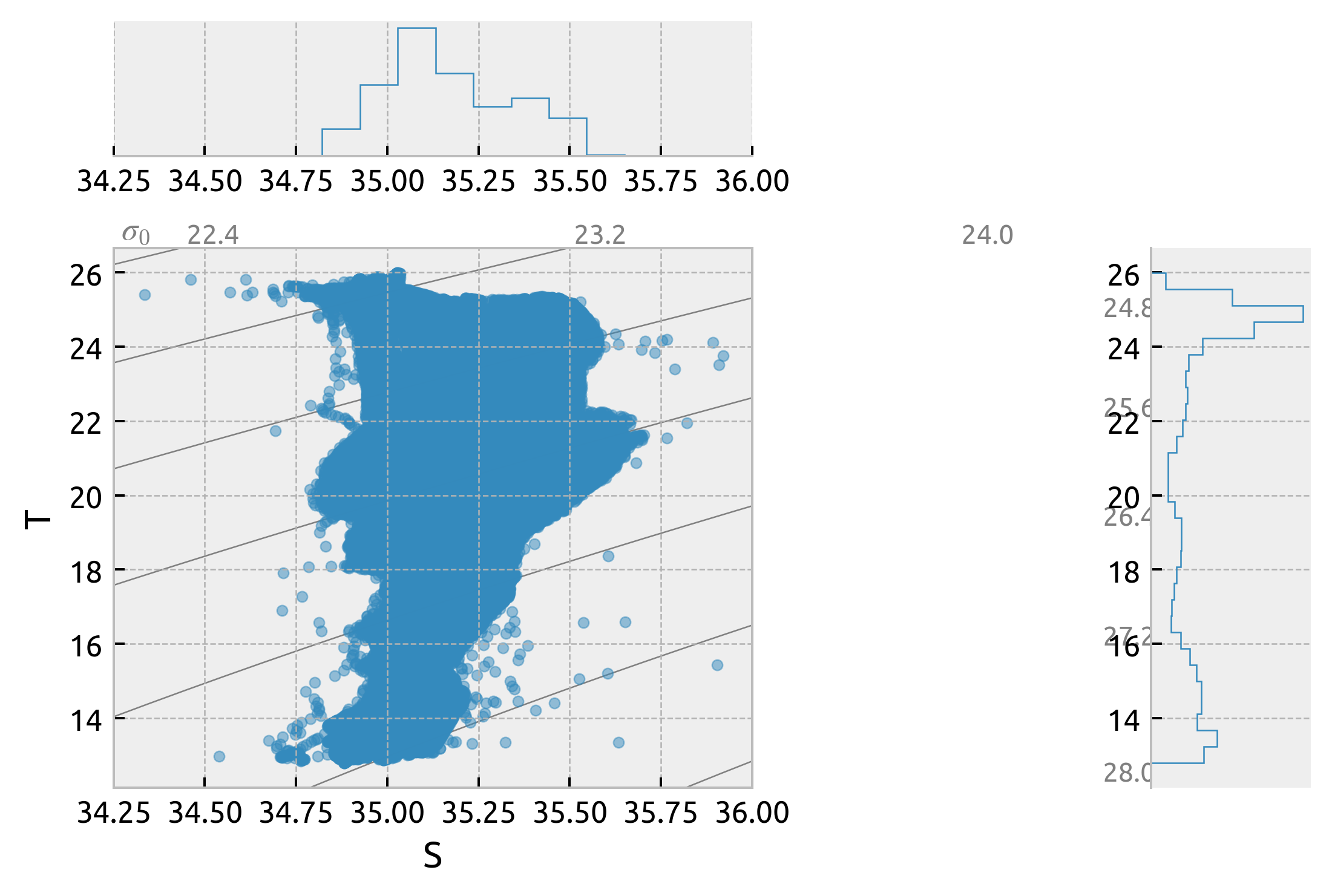
from matplotlib.lines import Line2D

ax = None
labels = []
lines = []
for label, group in tiwkegrouped:
    group = group.query(
        {"N_POINTS": "LATITUDE > 2 & LATITUDE < 6 & PRES > 35 & PRES < 100"}
    )
    hdl, axxx = dcpy.oceans.TSplot(group.PSAL, group.TEMP, kind="scatter", ax=ax)
    if ax is None:
        ax = axxx
    lines.append(Line2D([0], [0], color=hdl["Thist"][-1][0].get_edgecolor()))
    labels.append(label)

ax["s"].get_figure().legend(lines, labels, title="TIW KE", loc="upper right")

<matplotlib.legend.Legend at 0x7fd46c7bd6d0>

equix = xr.open_dataset("/home/deepak/datasets/microstructure/osu/equix.nc")

_, ax = dcpy.oceans.TSplot(equix.salt, equix.theta, hexbin=False)
ax["ts"].set_xlim([34.25, 36])

(34.25, 36.0)

argoclim = dcpy.oceans.read_argo_clim()
argoclim

<xarray.Dataset>
Dimensions:          (lat: 145, lon: 360, pres: 58, time: 180)
Coordinates:
  * lon              (lon) float32 20.5 21.5 22.5 23.5 ... 377.5 378.5 379.5
  * lat              (lat) float32 -64.5 -63.5 -62.5 -61.5 ... 77.5 78.5 79.5
  * pres             (pres) float32 2.5 10.0 20.0 ... 1.8e+03 1.9e+03 1.975e+03
  * time             (time) datetime64[ns] 2004-01-16 2004-02-15 ... 2018-09-29
Data variables:
    Tmean            (pres, lat, lon) float32 dask.array<chunksize=(58, 20, 60), meta=np.ndarray>
    Tanom            (time, pres, lat, lon) float32 dask.array<chunksize=(180, 58, 20, 60), meta=np.ndarray>
    BATHYMETRY_MASK  (pres, lat, lon) float32 dask.array<chunksize=(58, 20, 60), meta=np.ndarray>
    MAPPING_MASK     (pres, lat, lon) float32 dask.array<chunksize=(58, 20, 60), meta=np.ndarray>
    T                (time, pres, lat, lon) float32 dask.array<chunksize=(180, 58, 20, 60), meta=np.ndarray>
    Smean            (pres, lat, lon) float32 dask.array<chunksize=(58, 20, 60), meta=np.ndarray>
    Sanom            (time, pres, lat, lon) float32 dask.array<chunksize=(180, 58, 20, 60), meta=np.ndarray>
    S                (time, pres, lat, lon) float32 dask.array<chunksize=(180, 58, 20, 60), meta=np.ndarray>

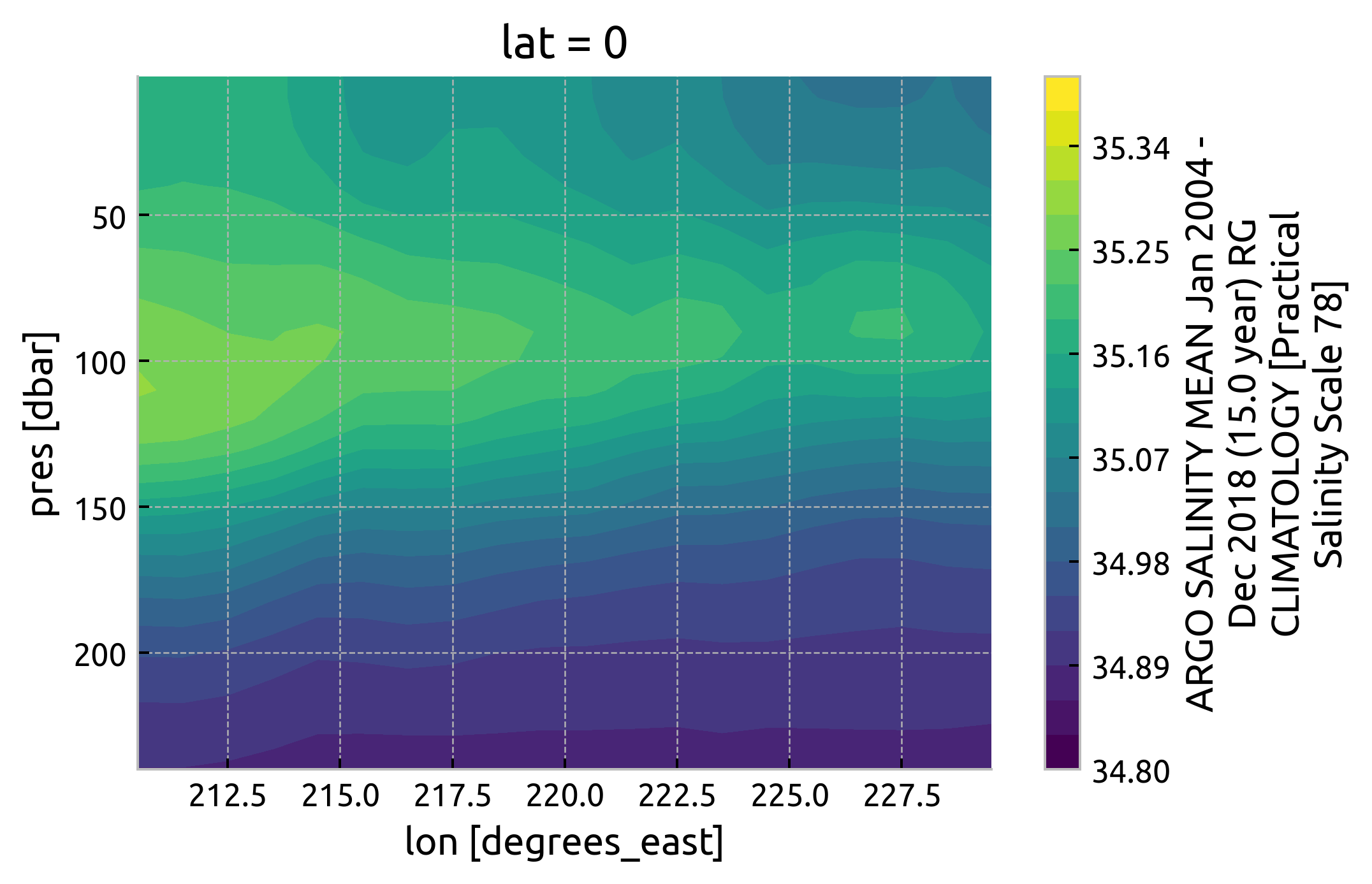
argoclim.Smean.interp(lat=0).sel(
    # lon=slice(165, 360 - 80),
    lon=slice(210, 230),
    pres=slice(250),
).cf.plot.contourf(levels=21, vmin=34.8, vmax=35.4)
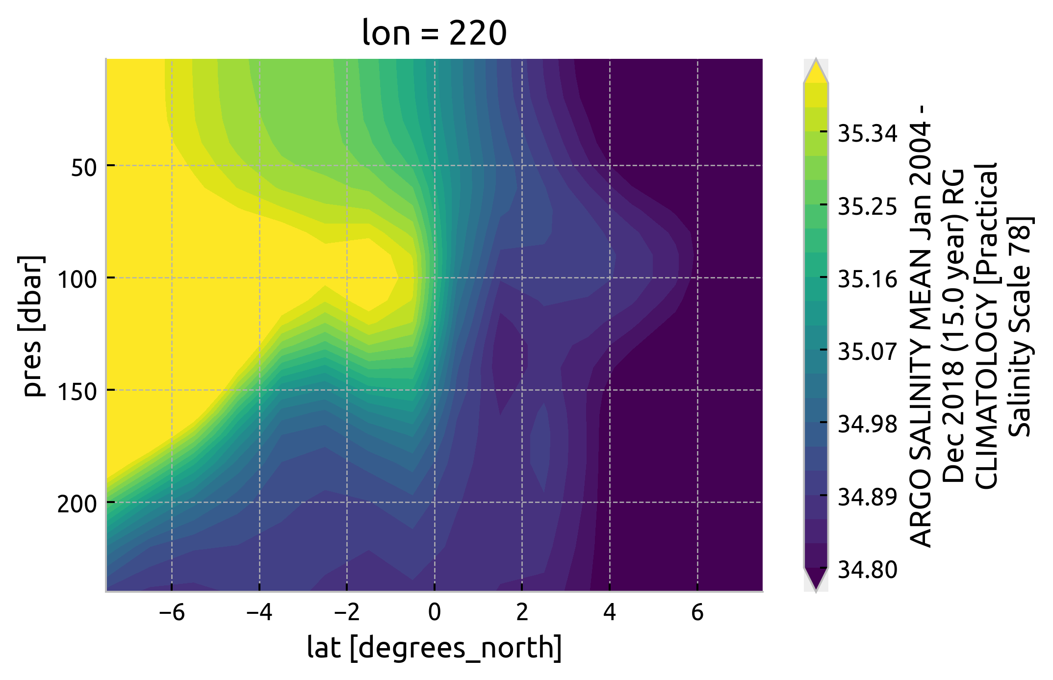
plt.figure()
argoclim.Smean.interp(lon=220).sel(lat=slice(-8, 8), pres=slice(250)).cf.plot.contourf(
    levels=21, vmin=34.8, vmax=35.4
)

<matplotlib.contour.QuadContourSet at 0x7fd4a331e640>

---

older T-S attempt

I first picked out three years 2008, 2010, 2015-16

ds = xr.open_mfdataset(
    ["argo_140_2008.nc", "argo_140_2010.nc", "argo_140_2016.nc"],
    preprocess=lambda ds: ds.drop_vars("N_POINTS"),
    concat_dim="N_POINTS",
    combine="nested",
)
ds

<xarray.Dataset>
Dimensions:                (N_POINTS: 62174)
Coordinates:
    LATITUDE               (N_POINTS) float64 dask.array<chunksize=(8464,), meta=np.ndarray>
    LONGITUDE              (N_POINTS) float64 dask.array<chunksize=(8464,), meta=np.ndarray>
    TIME                   (N_POINTS) datetime64[ns] dask.array<chunksize=(8464,), meta=np.ndarray>
Dimensions without coordinates: N_POINTS
Data variables: (12/13)
    CONFIG_MISSION_NUMBER  (N_POINTS) int64 dask.array<chunksize=(8464,), meta=np.ndarray>
    CYCLE_NUMBER           (N_POINTS) int64 dask.array<chunksize=(8464,), meta=np.ndarray>
    DATA_MODE              (N_POINTS) object dask.array<chunksize=(8464,), meta=np.ndarray>
    DIRECTION              (N_POINTS) object dask.array<chunksize=(8464,), meta=np.ndarray>
    PLATFORM_NUMBER        (N_POINTS) int64 dask.array<chunksize=(8464,), meta=np.ndarray>
    POSITION_QC            (N_POINTS) int64 dask.array<chunksize=(8464,), meta=np.ndarray>
    ...                     ...
    PRES_QC                (N_POINTS) int64 dask.array<chunksize=(8464,), meta=np.ndarray>
    PSAL                   (N_POINTS) float64 dask.array<chunksize=(8464,), meta=np.ndarray>
    PSAL_QC                (N_POINTS) int64 dask.array<chunksize=(8464,), meta=np.ndarray>
    TEMP                   (N_POINTS) float64 dask.array<chunksize=(8464,), meta=np.ndarray>
    TEMP_QC                (N_POINTS) int64 dask.array<chunksize=(8464,), meta=np.ndarray>
    TIME_QC                (N_POINTS) int64 dask.array<chunksize=(8464,), meta=np.ndarray>
Attributes:
    DATA_ID:              ARGO
    DOI:                  http://doi.org/10.17882/42182
    Fetched_from:         https://www.ifremer.fr/erddap
    Fetched_by:           deepak
    Fetched_date:         2021/04/02
    Fetched_constraints:  [x=-145.00/-135.00; y=-1.00/1.00; z=0.0/500.0; t=20...
    Fetched_uri:          https://www.ifremer.fr/erddap/tabledap/ArgoFloats.n...
    history:              Variables filtered according to DATA_MODE; Variable...

ds.TIME.dt.year.compute()

<xarray.DataArray 'year' (N_POINTS: 62174)>
array([2008, 2008, 2008, ..., 2016, 2016, 2016])
Coordinates:
    LATITUDE   (N_POINTS) float64 0.707 0.707 0.707 ... -0.202 -0.202 -0.202
    LONGITUDE  (N_POINTS) float64 -136.5 -136.5 -136.5 ... -135.6 -135.6 -135.6
    TIME       (N_POINTS) datetime64[ns] 2008-05-01T16:43:14 ... 2016-04-29T0...
Dimensions without coordinates: N_POINTS

ds.coords["year"] = ds.TIME.dt.year

sub = ds.query({"N_POINTS": "year == 2008"})
dcpy.oceans.TSplot(sub.PSAL, sub.TEMP, hexbin=False)

sub = ds.query({"N_POINTS": "year == 2010"})
dcpy.oceans.TSplot(sub.PSAL, sub.TEMP, hexbin=False)


sub = ds.query({"N_POINTS": "year == 2016"})
dcpy.oceans.TSplot(sub.PSAL, sub.TEMP, hexbin=False);

Download Argo data

from argopy import DataFetcher as ArgoDataFetcher

argo_loader = ArgoDataFetcher()

NATRE

ds = xr.open_mfdataset(
    "argo_natre_*.nc",
    preprocess=lambda ds: ds.drop_vars("N_POINTS"),
    concat_dim="N_POINTS",
    combine="nested",
).load()

ds.to_netcdf("../datasets/argo/natre.nc")

ds = argo_loader.region(
    [-35, -25, 23, 28, 0, 2000, "2005-01", "2010-12-31"]
).to_xarray()
ds.to_netcdf("argo_natre_2005_2010.nc")

ds = argo_loader.region(
    [-35, -25, 23, 28, 0, 2000, "2011-01", "2015-12-31"]
).to_xarray()
ds.to_netcdf("argo_natre_20010_2015.nc")

ds = argo_loader.region(
    [-35, -25, 23, 28, 0, 2000, "2016-01", "2020-12-31"]
).to_xarray()
ds.to_netcdf("argo_natre_2016_2020.nc")

TAO

ds = xr.open_mfdataset(
    "argo_140_20*_*.nc",
    preprocess=lambda ds: ds.drop_vars("N_POINTS"),
    concat_dim="N_POINTS",
    combine="nested",
).load()

ds.to_netcdf("../datasets/argo/tao.nc")

ds = argo_loader.region(
    [-145, -135, -2, 8, 0, 500, "2005-01", "2010-12-31"]
).to_xarray()
ds.to_netcdf("argo_140_2005_2010.nc")

ds = argo_loader.region(
    [-145, -135, -2, 8, 0, 500, "2011-01", "2015-12-31"]
).to_xarray()

ds.to_netcdf("argo_140_2011_2015.nc")

# Too much data end up getting HTTP 413: Payload too large errors.
for year in range(2016, 2021):
    ds = argo_loader.region(
        [-145, -135, -2, 8, 0, 500, f"{year}-01-01", f"{year}-12-31"]
    ).to_xarray()
    ds.to_netcdf(f"argo_140_{year}_{year}.nc")

---

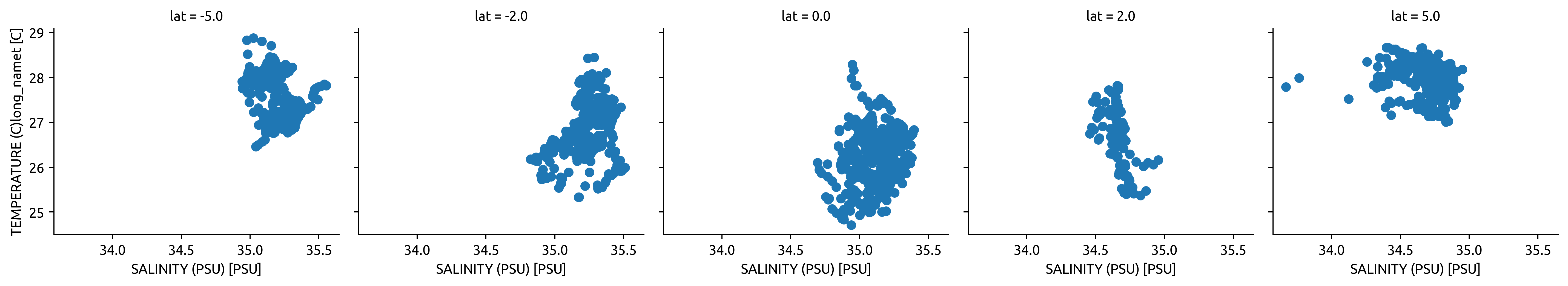
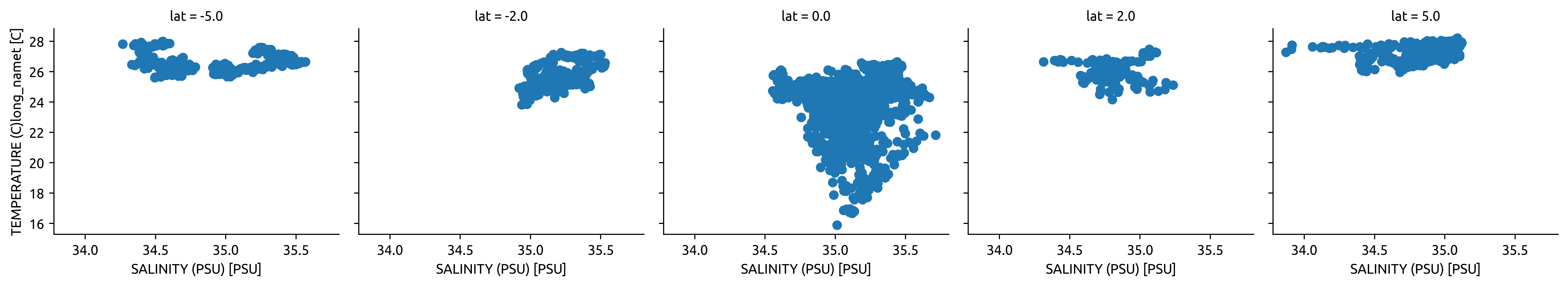
TAO mooring T-S

Conclusion There is not enough data. Basically no salinity observations off the equator.

import pump

temp = (
    xr.open_dataset("/home/deepak/TaoTritonPirataRama/TAO_TRITON/t_xyzt_dy.cdf")
    .rename({"T_20": "temp"})
    .cf.guess_coord_axis()
    .sel(lon=220)
)

salt = (
    xr.open_dataset("/home/deepak/TaoTritonPirataRama/TAO_TRITON/s_xyzt_dy.cdf")
    .rename({"S_41": "salt"})
    .cf.guess_coord_axis()
    .sel(lon=220)
)

tao = xr.merge([temp, salt], join="inner").sel(lat=[-5, -2, 0, 2, 5])
tao = tao.where(tao < 1000)

tao.sel(time="2003").plot.scatter("salt", "temp", col="lat")
tao.sel(time=slice("2008-Jun", "2009-Mar")).plot.scatter("salt", "temp", col="lat")

<xarray.plot.facetgrid.FacetGrid at 0x7f78fe81bee0>