Mixing below EUC

%load_ext watermark
%matplotlib inline


import dcpy
import dcpy.eos
import holoviews as hv
import matplotlib as mpl
import numpy as np
from datatree import DataTree

import xarray as xr
from pump import mixpods

hv.notebook_extension("bokeh")


xr.set_options(keep_attrs=True)
mpl.rcParams["figure.dpi"] = 140
%watermark -iv

holoviews : 1.14.8
pump      : 0.1
dcpy      : 0.2.1.dev45+g67ec22a.d20230504
numpy     : 1.23.5
xarray    : 2023.3.0
matplotlib: 3.6.3

equix = xr.open_dataset("~/datasets/microstructure/osu/equix.nc")
tiwe = xr.open_dataset("~/datasets/microstructure/osu/tiwe.nc")
equix.attrs["name"] = "EQUIX"
tiwe["Sh2"] = tiwe.u.differentiate("depth") ** 2 + tiwe.v.differentiate("depth") ** 2
tiwe["Sh2"] = tiwe.u.differentiate("depth") ** 2 + tiwe.v.differentiate("depth") ** 2


tree = DataTree.from_dict({"TIWE": tiwe, "EQUIX": equix})


edges = np.arange(-202.5, 202.5, 5)

EUC maximum

EUC is moving by 20m or so

mixpods.map_hvplot(
    lambda ds, name, muted: ds["eucmax"]
    .assign_coords(time=ds["time"] - ds["time"][0])
    .hvplot.line(x="time", label=name, muted=muted),
    tree,
)

Bin to EUC-coordinate

for name, node in tree.children.items():
    binned = (
        node.ds[["u", "v", "chi", "eps", "theta"]]
        .assign_coords(zeuc=node.ds["eucmax"] - node.ds["depth"])
        .groupby_bins("zeuc", bins=edges, labels=node["zeuc"].data)
        .mean("depth", method="map-reduce")
        .rename({"zeuc_bins": "zeuc"})
    )
    binned["Sh2"] = (
        binned.u.differentiate("zeuc") ** 2 + binned.v.differentiate("zeuc") ** 2
    )
    binned["Tz"] = binned["theta"].differentiate("zeuc")
    binned["N2T"] = (
        9.81
        * dcpy.eos.alpha(35, binned.theta, binned.zeuc, pt=True).mean("time")
        * binned["theta"].differentiate("zeuc")
    )
    binned["Rig_T"] = binned.N2T / binned.Sh2
    binned["Shred2"] = binned.Sh2 - 4 * binned.N2T
    binned["KT"] = (
        binned.chi / 2 / binned.Tz.where(np.abs(binned.Tz) > 1e-4) ** 2
    ).assign_attrs(long_name="KT")
    binned["ν"] = (binned.eps / binned.Sh2.where(binned.Sh2 > 1e-5)).assign_attrs(
        long_name="ν"
    )
    tree[f"{name}/euc"] = DataTree(binned)

Mixing below the EUC

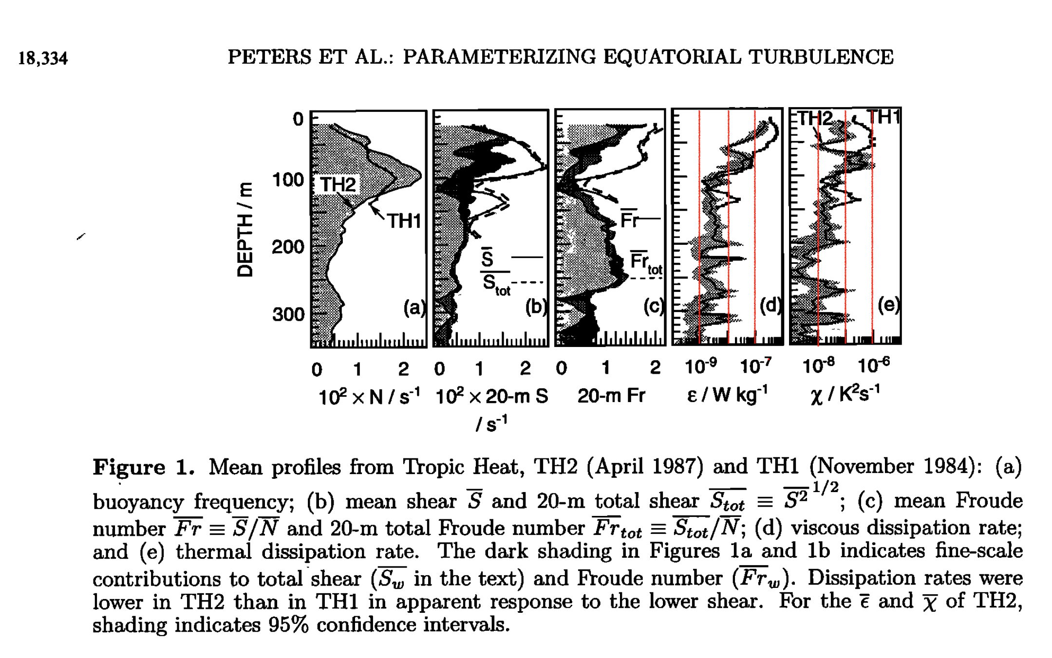
1. Below the EUC, TIWE (days 308-328) and EQUIX are quite similar.

2. ν ~ 1e-4, \(K_T\) > 1e-5,

3. \(ε\) ~ 1e-8 (matches with TH2, Peters et al, 1995). Peters et al, 1995 say mixing was intermittent and the mean dominated by rare events below the EUC max.

4. Rig_T was calculated after regridding to EUC-centered coordinate.

TODO

• add to mixpods

• Look at Ri

import dcpy.datatree

euc = tree.dc.extract_leaf("euc")

h = {
    varname: mixpods.map_hvplot(
        lambda node, name, muted: node.ds[varname]
        .reset_coords(drop=True)
        .hvplot.line(ylabel=varname, label=name, logx=varname != "u", invert=True),
        euc.dc.subset_nodes(varname).mean("time"),
    )
    for varname in ["u", "chi", "eps", "KT", "ν"]
}
h["chi"].opts(ylim=(1e-9, 1e-4))
h["eps"].opts(ylim=(1e-9, 1e-4))
h["KT"].opts(ylim=(1e-6, 3))
h["ν"].opts(ylim=(1e-6, 1e-1));

h2 = {
    varname: mixpods.map_hvplot(
        lambda node, name, muted: node.ds[varname]
        .reset_coords(drop=True)
        .hvplot.line(ylabel=varname, label=name, logx=False, invert=True),
        euc.dc.subset_nodes(varname).median("time"),
    )
    for varname in ["Rig_T"]
}

hv.Layout(list(h.values()) + [h2["Rig_T"].opts(ylim=(0, 5))]).opts(
    hv.opts.Curve(frame_width=150, frame_height=300, xlim=(-150, 150)),
    hv.opts.Layout(shared_axes=True),
    hv.opts.Overlay(show_legend=True, show_grid=True, legend_position="top"),
).cols(6)

def plot_turb_diags(node):
    ds = node.ds.resample(time="H").mean()

    return (
        (
            ds.Shred2.hvplot.quadmesh(
                title="Sh_red^2", x="time", cmap="coolwarm", clim=(-1e-4, 1e-4)
            )
            + ds.eps.hvplot.quadmesh(
                title="ε", clim=(1e-9, 1e-6), cmap="fire", cnorm="log", x="time"
            )
            + ds.Rig_T.hvplot.quadmesh(title="Rig_T", x="time", clim=(0.1, 1))
        )
        .cols(1)
        .opts(hv.opts.QuadMesh(frame_width=900, frame_height=200))
    )

Tropic Heat 2

from IPython.display import Image

Image("../images/peters-1995-TH2-mean-profiles.png", width=1200)

Holmes et al 2016

Large temperature variance dissipation 𝜒 > 10−7 K2 s−1 (Figures 1a and 1b) occurs in the upper 250 m, particularly near the equator, associated with upper ocean mixing processes such as shear instability in the Equatorial Undercurrent [Gregg et al., 1985]. Enhanced 𝜒 ∼ 10−9 K2 s−1 occurs between 250 m and 1000 m and generally small 𝜒<10−9 K2 s−1 occurs below 1000 m. However, there is a region of large 𝜒 peaking at 10−8 K2 s−1 at 1/2∘S between 3200 m and the seafloor (Figure 1b). There is also evidence of enhanced 𝜒 reaching 10−9 K2 s−1 close to the seafloor.

TIWE

plot_turb_diags(euc["TIWE"])

EQUIX

plot_turb_diags(euc["EQUIX"])