TIW vertical velocity in MITgcm simulations#
TODO:
Conditional average by TIW KE?
look more closely at downwelling in 2008 OND
regrid to ML-relative vertical coordinate; not necessary MLD seems quite small!
average 2005,2006; and then 2008, 2009 because they look similar
better season definition: based on TIWKE?
Show code cell content
# %load_ext %autoreload
%autoreload 1
%matplotlib inline
%config InlineBackend.figure_format="retina"
import cf_xarray
import dask
import dcpy
import distributed
import holoviews as hv
import hvplot.xarray
import matplotlib as mpl
import matplotlib.dates as mdates
import matplotlib.pyplot as plt
import matplotlib.units as munits
import numpy as np
import pandas as pd
import panel.widgets as pnw
import seawater as sw
import xarray as xr
import xgcm
from holoviews import opts
%aimport pump
mpl.rcParams["figure.dpi"] = 140
mpl.rcParams["savefig.dpi"] = 300
mpl.rcParams["savefig.bbox"] = "tight"
munits.registry[np.datetime64] = mdates.ConciseDateConverter()
xr.set_options(keep_attrs=True)
hv.extension("bokeh")
# hv.opts.defaults(opts.Image(fontscale=1.5), opts.Curve(fontscale=1.5))
print(dask.__version__)
print(distributed.__version__)
print(xr.__version__)
xr.DataArray([1.0])


2021.07.2
2021.07.2
0.19.0
<xarray.DataArray (dim_0: 1)> array([1.]) Dimensions without coordinates: dim_0
- dim_0: 1
- 1.0
array([1.])
Show code cell content
import dask_jobqueue
if "client" in locals():
client.close()
# if "cluster" in locals():
# cluster.close()
env = {"OMP_NUM_THREADS": "1", "NUMBA_NUM_THREADS": "1", "OPENBLAS_NUM_THREADS": "1"}
# cluster = distributed.LocalCluster(
# n_workers=8,
# threads_per_worker=1,
# env=env
# )
if "cluster" in locals():
del cluster
# cluster = ncar_jobqueue.NCARCluster(
# account="NCGD0011",
# scheduler_options=dict(dashboard_address=":9797"),
# env_extra=env,
# )
cluster = dask_jobqueue.PBSCluster(
cores=1, # The number of cores you want
memory="23GB", # Amount of memory
processes=1, # How many processes
queue="casper", # The type of queue to utilize (/glade/u/apps/dav/opt/usr/bin/execcasper)
local_directory="$TMPDIR", # Use your local directory
resource_spec="select=1:ncpus=1:mem=23GB", # Specify resources
project="ncgd0011", # Input your project ID here
walltime="02:00:00", # Amount of wall time
interface="ib0", # Interface to use
)
cluster.scale(6)
Show code cell content
cluster.scale(24)
Show code cell content
client = distributed.Client(cluster)
client
Client
Client-1880c442-116b-11ec-b9b4-3cecef1b11de
| Connection method: Cluster object | Cluster type: PBSCluster |
| Dashboard: /proxy/8787/status |
Cluster Info
PBSCluster
9890abbc
| Dashboard: /proxy/8787/status | Workers: 0 |
| Total threads: 0 | Total memory: 0 B |
Scheduler Info
Scheduler
Scheduler-d3bda136-da83-427c-ab64-b71d1165a748
| Comm: tcp://10.12.206.51:45967 | Workers: 0 |
| Dashboard: /proxy/8787/status | Total threads: 0 |
| Started: Just now | Total memory: 0 B |
Workers
Means#
ds, metrics = pump.model.read_mitgcm_20_year(
state=True, start="2008-01-01", stop="2017-12-31"
)
ds
seasonalmean = ds.resample(time="QS").mean()
seasonalmean
<xarray.Dataset>
Dimensions: (time: 68, RF: 136, YG: 400, XG: 1420, YC: 400, XC: 1420, RC: 136)
Coordinates:
* time (time) datetime64[ns] 2001-01-01 2001-04-01 ... 2017-10-01
* RF (RF) float64 0.0 -2.5 -5.0 -7.5 ... -797.0 -851.7 -911.6
* YG (YG) float64 -10.0 -9.95 -9.9 -9.85 ... 9.8 9.85 9.9 9.95
* XG (XG) float64 -168.0 -168.0 -167.9 ... -97.18 -97.12 -97.08
* YC (YC) float64 -9.975 -9.925 -9.875 ... 9.875 9.925 9.975
* XC (XC) float64 -168.0 -167.9 -167.9 ... -97.15 -97.1 -97.05
* RC (RC) float64 -1.25 -3.75 -6.25 ... -824.4 -881.7 -944.4
Data variables:
theta (time, RC, YC, XC) float32 dask.array<chunksize=(1, 136, 400, 500), meta=np.ndarray>
u (time, RC, YC, XG) float32 dask.array<chunksize=(1, 136, 400, 500), meta=np.ndarray>
v (time, RC, YG, XC) float32 dask.array<chunksize=(1, 136, 400, 500), meta=np.ndarray>
w (time, RF, YC, XC) float32 dask.array<chunksize=(1, 136, 400, 500), meta=np.ndarray>
salt (time, RC, YC, XC) float32 dask.array<chunksize=(1, 136, 400, 500), meta=np.ndarray>
KPP_diffusivity (time, RF, YC, XC) float32 dask.array<chunksize=(1, 136, 400, 500), meta=np.ndarray>
dens (time, RC, YC, XC) float32 dask.array<chunksize=(1, 136, 400, 500), meta=np.ndarray>
Attributes:
title: daily snapshot from 1/20 degree Equatorial Pacific MI...
easting: longitude
northing: latitude
field_julian_date: 447072
julian_day_unit: days since 1950-01-01 00:00:00- time: 68
- RF: 136
- YG: 400
- XG: 1420
- YC: 400
- XC: 1420
- RC: 136
- time(time)datetime64[ns]2001-01-01 ... 2017-10-01
array(['2001-01-01T00:00:00.000000000', '2001-04-01T00:00:00.000000000', '2001-07-01T00:00:00.000000000', '2001-10-01T00:00:00.000000000', '2002-01-01T00:00:00.000000000', '2002-04-01T00:00:00.000000000', '2002-07-01T00:00:00.000000000', '2002-10-01T00:00:00.000000000', '2003-01-01T00:00:00.000000000', '2003-04-01T00:00:00.000000000', '2003-07-01T00:00:00.000000000', '2003-10-01T00:00:00.000000000', '2004-01-01T00:00:00.000000000', '2004-04-01T00:00:00.000000000', '2004-07-01T00:00:00.000000000', '2004-10-01T00:00:00.000000000', '2005-01-01T00:00:00.000000000', '2005-04-01T00:00:00.000000000', '2005-07-01T00:00:00.000000000', '2005-10-01T00:00:00.000000000', '2006-01-01T00:00:00.000000000', '2006-04-01T00:00:00.000000000', '2006-07-01T00:00:00.000000000', '2006-10-01T00:00:00.000000000', '2007-01-01T00:00:00.000000000', '2007-04-01T00:00:00.000000000', '2007-07-01T00:00:00.000000000', '2007-10-01T00:00:00.000000000', '2008-01-01T00:00:00.000000000', '2008-04-01T00:00:00.000000000', '2008-07-01T00:00:00.000000000', '2008-10-01T00:00:00.000000000', '2009-01-01T00:00:00.000000000', '2009-04-01T00:00:00.000000000', '2009-07-01T00:00:00.000000000', '2009-10-01T00:00:00.000000000', '2010-01-01T00:00:00.000000000', '2010-04-01T00:00:00.000000000', '2010-07-01T00:00:00.000000000', '2010-10-01T00:00:00.000000000', '2011-01-01T00:00:00.000000000', '2011-04-01T00:00:00.000000000', '2011-07-01T00:00:00.000000000', '2011-10-01T00:00:00.000000000', '2012-01-01T00:00:00.000000000', '2012-04-01T00:00:00.000000000', '2012-07-01T00:00:00.000000000', '2012-10-01T00:00:00.000000000', '2013-01-01T00:00:00.000000000', '2013-04-01T00:00:00.000000000', '2013-07-01T00:00:00.000000000', '2013-10-01T00:00:00.000000000', '2014-01-01T00:00:00.000000000', '2014-04-01T00:00:00.000000000', '2014-07-01T00:00:00.000000000', '2014-10-01T00:00:00.000000000', '2015-01-01T00:00:00.000000000', '2015-04-01T00:00:00.000000000', '2015-07-01T00:00:00.000000000', '2015-10-01T00:00:00.000000000', '2016-01-01T00:00:00.000000000', '2016-04-01T00:00:00.000000000', '2016-07-01T00:00:00.000000000', '2016-10-01T00:00:00.000000000', '2017-01-01T00:00:00.000000000', '2017-04-01T00:00:00.000000000', '2017-07-01T00:00:00.000000000', '2017-10-01T00:00:00.000000000'], dtype='datetime64[ns]') - RF(RF)float640.0 -2.5 -5.0 ... -851.7 -911.6
array([ 0. , -2.5 , -5. , -7.5 , -10. , -12.5 , -15. , -17.5 , -20. , -22.5 , -25. , -27.5 , -30. , -32.5 , -35. , -37.5 , -40. , -42.5 , -45. , -47.5 , -50. , -52.5 , -55. , -57.5 , -60. , -62.5 , -65. , -67.5 , -70. , -72.5 , -75. , -77.5 , -80. , -82.5 , -85. , -87.5 , -90. , -92.5 , -95. , -97.5 , -100. , -102.5 , -105. , -107.5 , -110. , -112.5 , -115. , -117.5 , -120. , -122.5 , -125. , -127.5 , -130. , -132.5 , -135. , -137.5 , -140. , -142.5 , -145. , -147.5 , -150. , -152.5 , -155. , -157.5 , -160. , -162.5 , -165. , -167.5 , -170. , -172.5 , -175. , -177.5 , -180. , -182.5 , -185. , -187.5 , -190. , -192.5 , -195. , -197.5 , -200. , -202.5 , -205. , -207.5 , -210. , -212.5 , -215. , -217.5 , -220. , -222.5 , -225. , -227.5 , -230. , -232.5 , -235. , -237.5 , -240. , -242.5 , -245. , -247.5 , -250. , -252.737503, -255.735107, -259.017395, -262.611603, -266.547211, -270.856689, -275.575592, -280.742798, -286.400909, -292.596497, -299.380615, -306.809204, -314.943604, -323.850708, -333.604004, -344.283905, -355.978394, -368.783813, -382.805695, -398.159698, -414.972412, -433.382294, -453.541107, -475.61499 , -499.785889, -526.252991, -555.234497, -586.969299, -621.718872, -659.769714, -701.435303, -747.059082, -797.017212, -851.721313, -911.622314]) - YG(YG)float64-10.0 -9.95 -9.9 ... 9.85 9.9 9.95
array([-10. , -9.95, -9.9 , ..., 9.85, 9.9 , 9.95])
- XG(XG)float64-168.0 -168.0 ... -97.12 -97.08
array([-168.025 , -167.975 , -167.925 , ..., -97.175002, -97.124998, -97.075003]) - YC(YC)float64-9.975 -9.925 ... 9.925 9.975
- axis :
- Y
array([-9.975, -9.925, -9.875, ..., 9.875, 9.925, 9.975])
- XC(XC)float64-168.0 -167.9 ... -97.1 -97.05
- axis :
- X
array([-168. , -167.95 , -167.9 , ..., -97.15 , -97.099997, -97.050002]) - RC(RC)float64-1.25 -3.75 -6.25 ... -881.7 -944.4
- axis :
- Z
array([ -1.25 , -3.75 , -6.25 , -8.75 , -11.25 , -13.75 , -16.25 , -18.75 , -21.25 , -23.75 , -26.25 , -28.75 , -31.25 , -33.75 , -36.25 , -38.75 , -41.25 , -43.75 , -46.25 , -48.75 , -51.25 , -53.75 , -56.25 , -58.75 , -61.25 , -63.75 , -66.25 , -68.75 , -71.25 , -73.75 , -76.25 , -78.75 , -81.25 , -83.75 , -86.25 , -88.75 , -91.25 , -93.75 , -96.25 , -98.75 , -101.25 , -103.75 , -106.25 , -108.75 , -111.25 , -113.75 , -116.25 , -118.75 , -121.25 , -123.75 , -126.25 , -128.75 , -131.25 , -133.75 , -136.25 , -138.75 , -141.25 , -143.75 , -146.25 , -148.75 , -151.25 , -153.75 , -156.25 , -158.75 , -161.25 , -163.75 , -166.25 , -168.75 , -171.25 , -173.75 , -176.25 , -178.75 , -181.25 , -183.75 , -186.25 , -188.75 , -191.25 , -193.75 , -196.25 , -198.75 , -201.25 , -203.75 , -206.25 , -208.75 , -211.25 , -213.75 , -216.25 , -218.75 , -221.25 , -223.75 , -226.25 , -228.75 , -231.25 , -233.75 , -236.25 , -238.75 , -241.25 , -243.75 , -246.25 , -248.75 , -251.368744, -254.236298, -257.376251, -260.814514, -264.579407, -268.701935, -273.216156, -278.15921 , -283.571838, -289.498688, -295.988556, -303.09491 , -310.876404, -319.397156, -328.727356, -338.943939, -350.131165, -362.381104, -375.794739, -390.482697, -406.56604 , -424.177338, -443.4617 , -464.578064, -487.700439, -513.01947 , -540.743774, -571.101929, -604.344116, -640.744324, -680.602478, -724.247192, -772.038147, -824.369263, -881.671814, -944.418091])
- theta(time, RC, YC, XC)float32dask.array<chunksize=(1, 136, 400, 500), meta=np.ndarray>
Array Chunk Bytes 19.57 GiB 103.76 MiB Shape (68, 136, 400, 1420) (1, 136, 400, 500) Count 87653 Tasks 204 Chunks Type float32 numpy.ndarray - u(time, RC, YC, XG)float32dask.array<chunksize=(1, 136, 400, 500), meta=np.ndarray>
Array Chunk Bytes 19.57 GiB 103.76 MiB Shape (68, 136, 400, 1420) (1, 136, 400, 500) Count 87653 Tasks 204 Chunks Type float32 numpy.ndarray - v(time, RC, YG, XC)float32dask.array<chunksize=(1, 136, 400, 500), meta=np.ndarray>
Array Chunk Bytes 19.57 GiB 103.76 MiB Shape (68, 136, 400, 1420) (1, 136, 400, 500) Count 87653 Tasks 204 Chunks Type float32 numpy.ndarray - w(time, RF, YC, XC)float32dask.array<chunksize=(1, 136, 400, 500), meta=np.ndarray>
Array Chunk Bytes 19.57 GiB 103.76 MiB Shape (68, 136, 400, 1420) (1, 136, 400, 500) Count 87653 Tasks 204 Chunks Type float32 numpy.ndarray - salt(time, RC, YC, XC)float32dask.array<chunksize=(1, 136, 400, 500), meta=np.ndarray>
Array Chunk Bytes 19.57 GiB 103.76 MiB Shape (68, 136, 400, 1420) (1, 136, 400, 500) Count 87653 Tasks 204 Chunks Type float32 numpy.ndarray - KPP_diffusivity(time, RF, YC, XC)float32dask.array<chunksize=(1, 136, 400, 500), meta=np.ndarray>
Array Chunk Bytes 19.57 GiB 103.76 MiB Shape (68, 136, 400, 1420) (1, 136, 400, 500) Count 87653 Tasks 204 Chunks Type float32 numpy.ndarray - dens(time, RC, YC, XC)float32dask.array<chunksize=(1, 136, 400, 500), meta=np.ndarray>
Array Chunk Bytes 19.57 GiB 103.76 MiB Shape (68, 136, 400, 1420) (1, 136, 400, 500) Count 186998 Tasks 204 Chunks Type float32 numpy.ndarray
- title :
- daily snapshot from 1/20 degree Equatorial Pacific MITgcm simulation
- easting :
- longitude
- northing :
- latitude
- field_julian_date :
- 447072
- julian_day_unit :
- days since 1950-01-01 00:00:00
dcpy.dask.batch_to_zarr(
seasonalmean[["u", "theta"]],
file="/glade/work/dcherian/pump/zarrs/seasonalutheta.zarr",
batch_size=12,
dim="time",
)
100%|██████████| 6/6 [20:23<00:00, 203.96s/it]
cluster.scale(12)
v = dcpy.dask.map_copy(ds.v.sel(RC=slice(-80)).sel(XC=-140, YG=0, method="nearest"))
v = v.load()
v.RC.attrs["axis"] = "Z"
v.to_dataset().to_zarr("/glade/work/dcherian/pump/zarrs/v-0-140-80m.zarr")
<xarray.backends.zarr.ZarrStore at 0x2ba17e0f3ba0>
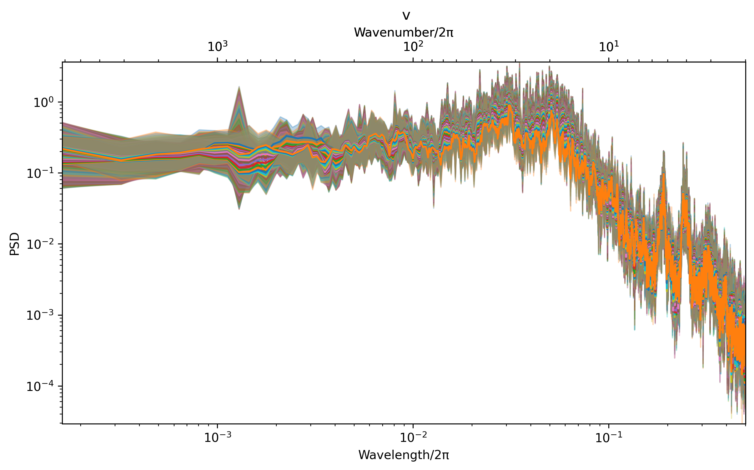
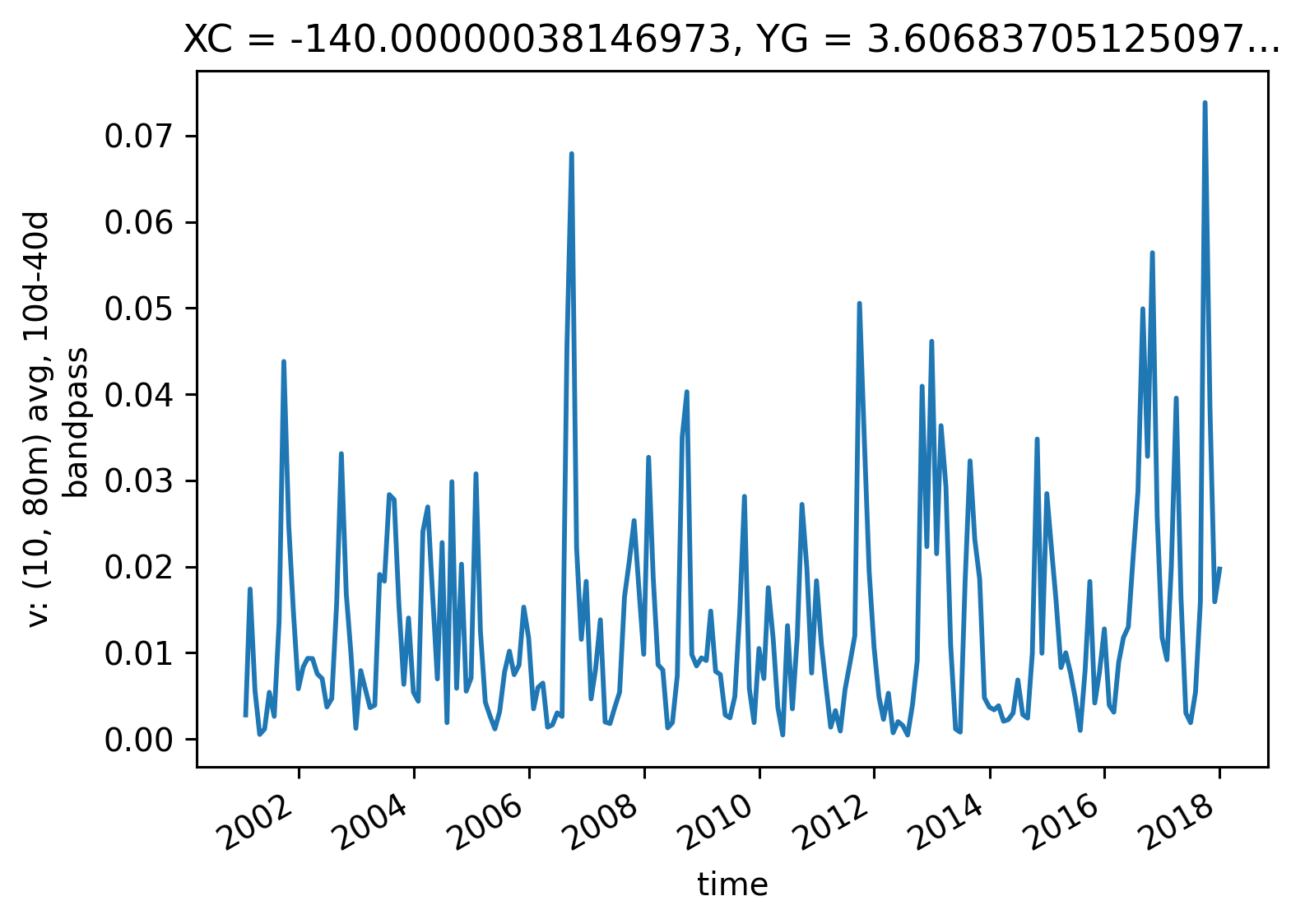
TIWKE#
make TIW KE proxy for later conditional averaging
def tiw_avg_filter_v(v):
import xfilter
v = xfilter.bandpass(
v.cf.sel(Z=slice(-10, -80)).cf.mean("Z"),
coord="time",
freq=[1 / 10.0, 1 / 50.0],
cycles_per="D",
method="pad",
num_discard=0,
order=3,
)
if v.count() == 0:
raise ValueError("No good data in filtered depth-averaged v.")
v.attrs["long_name"] = "v: (10, 80m) avg, 10d-40d bandpass"
return v
# tiwv = tiw_avg_filter_v(v)
dcpy.ts.PlotSpectrum(v)
([<matplotlib.lines.Line2D at 0x2ba1f7dc9460>,
<matplotlib.lines.Line2D at 0x2ba1f2f34b50>,
<matplotlib.lines.Line2D at 0x2ba1f6d644f0>,
<matplotlib.lines.Line2D at 0x2ba1f2f34e50>,
<matplotlib.lines.Line2D at 0x2ba1f2f34310>,
<matplotlib.lines.Line2D at 0x2ba1fc7fc940>,
<matplotlib.lines.Line2D at 0x2ba1fd14f250>,
<matplotlib.lines.Line2D at 0x2ba1fcea8610>,
<matplotlib.lines.Line2D at 0x2ba20e8b7040>,
<matplotlib.lines.Line2D at 0x2ba1fc26d940>,
<matplotlib.lines.Line2D at 0x2ba181a6c190>,
<matplotlib.lines.Line2D at 0x2ba1fe1d8ee0>,
<matplotlib.lines.Line2D at 0x2ba0d09da340>,
<matplotlib.lines.Line2D at 0x2ba2122b1a00>,
<matplotlib.lines.Line2D at 0x2ba210695460>,
<matplotlib.lines.Line2D at 0x2ba20f1e6190>,
<matplotlib.lines.Line2D at 0x2ba1f69d09d0>,
<matplotlib.lines.Line2D at 0x2ba1fca98460>,
<matplotlib.lines.Line2D at 0x2ba1fe122100>,
<matplotlib.lines.Line2D at 0x2ba0d09da2e0>,
<matplotlib.lines.Line2D at 0x2ba1f7c02850>,
<matplotlib.lines.Line2D at 0x2ba2122b1820>,
<matplotlib.lines.Line2D at 0x2ba1fcea87f0>,
<matplotlib.lines.Line2D at 0x2ba1fcb76700>,
<matplotlib.lines.Line2D at 0x2ba1f68f3a30>,
<matplotlib.lines.Line2D at 0x2ba1fc7d4a00>,
<matplotlib.lines.Line2D at 0x2ba1a7db2310>,
<matplotlib.lines.Line2D at 0x2ba20c1c7c70>,
<matplotlib.lines.Line2D at 0x2ba1fc7235b0>,
<matplotlib.lines.Line2D at 0x2ba1fc26d640>,
<matplotlib.lines.Line2D at 0x2ba1fc7238b0>,
<matplotlib.lines.Line2D at 0x2ba1fc7d4370>],
<AxesSubplot:title={'center':' v'}, xlabel='Wavelength/2π', ylabel='PSD'>)
tiwke = dask_groupby.xarray.resample_reduce(
(tiwv**2 / 2).resample(time="M"), func="mean"
)
tiwke.plot()
[<matplotlib.lines.Line2D at 0x2ba2138bb370>]
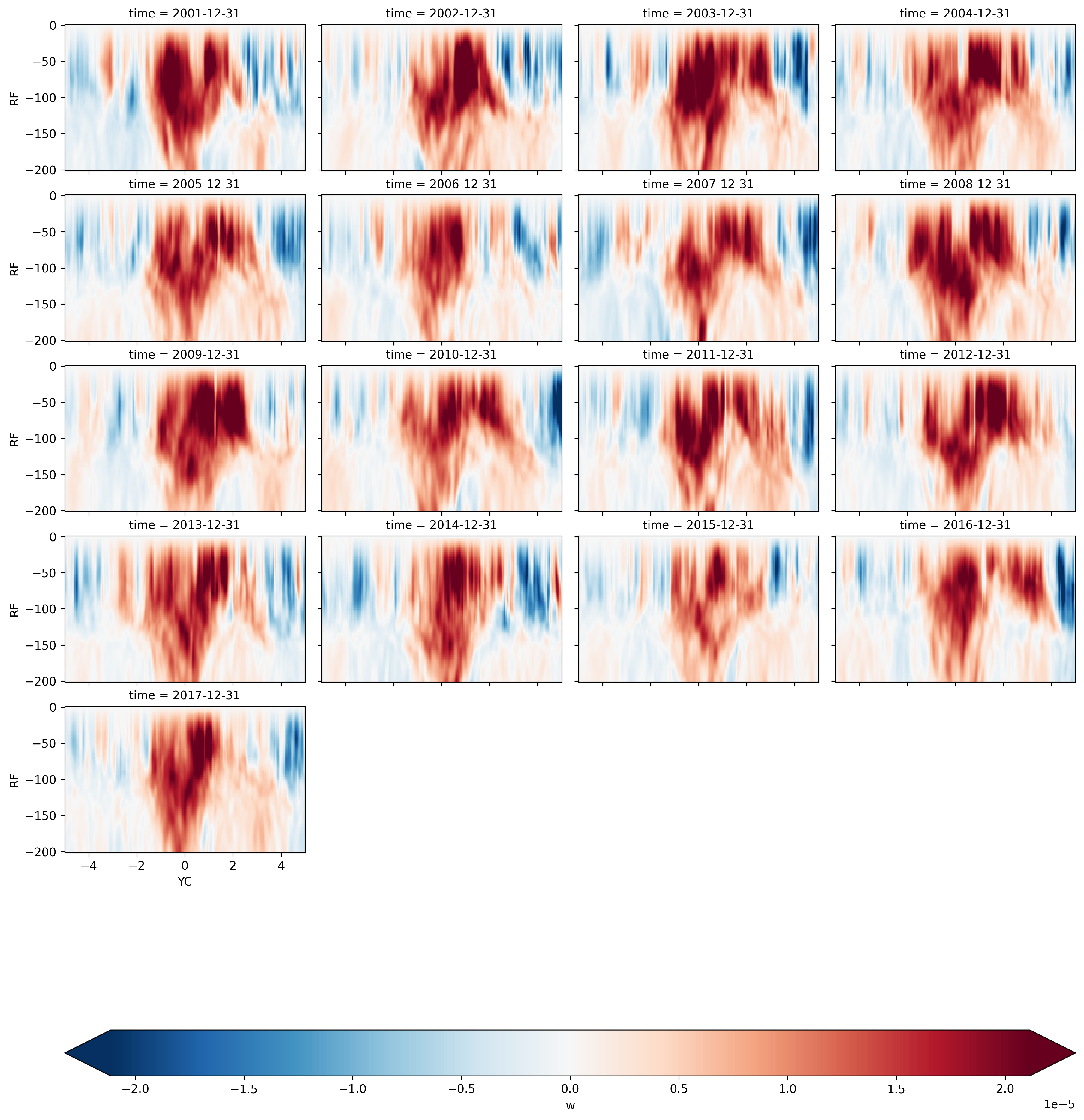
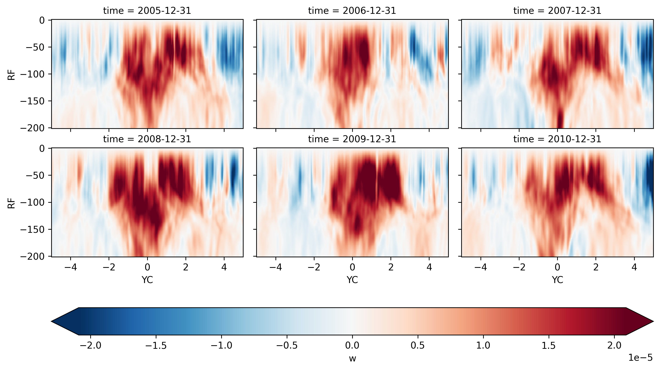
Annual means#
wmean = xr.open_zarr("meanw.zarr")
wmean.sel(XC=-140, method="nearest").sel(YC=slice(-5, 5), RF=slice(-200)).w.plot(
col="time",
col_wrap=4,
y="RF",
x="YC",
robust=True,
cmap="RdBu_r",
cbar_kwargs={"orientation": "horizontal"},
)
<xarray.plot.facetgrid.FacetGrid at 0x2ba0d082a5e0>
wmean.sel(XC=-140, method="nearest").sel(YC=slice(-5, 5), RF=slice(-200)).w.plot(
col="time",
col_wrap=3,
y="RF",
x="YC",
robust=True,
cmap="RdBu_r",
cbar_kwargs={"orientation": "horizontal"},
)
<xarray.plot.facetgrid.FacetGrid at 0x2b8a6f5464f0>
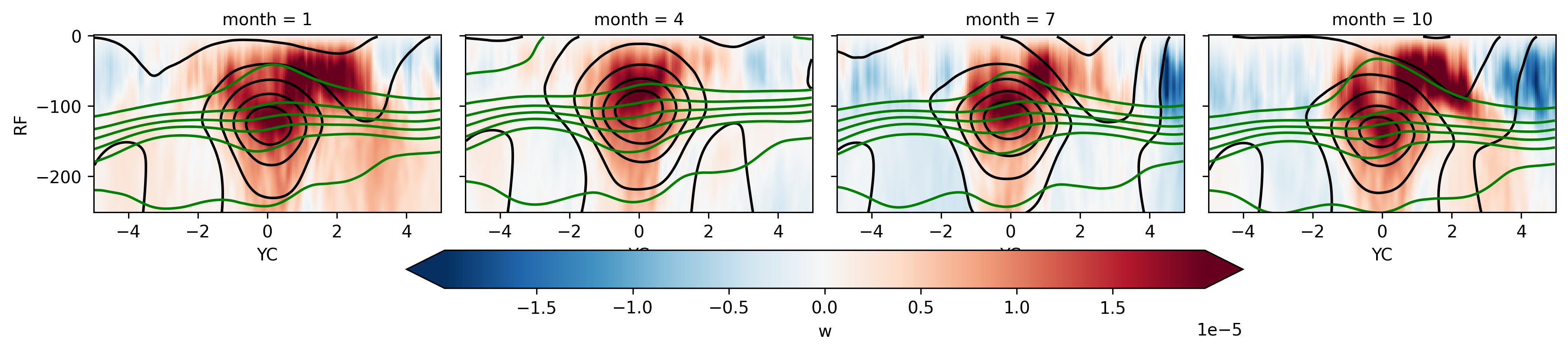
Seasonal mean#
Show code cell content
seasonalmean = xr.open_mfdataset("/glade/work/dcherian/pump/zarrs/seasonal*.zarr")
seasonalmean
/glade/u/home/dcherian/miniconda3/envs/dcpy/lib/python3.8/site-packages/xarray/backends/plugins.py:110: RuntimeWarning: 'netcdf4' fails while guessing
warnings.warn(f"{engine!r} fails while guessing", RuntimeWarning)
/glade/u/home/dcherian/miniconda3/envs/dcpy/lib/python3.8/site-packages/xarray/backends/plugins.py:110: RuntimeWarning: 'h5netcdf' fails while guessing
warnings.warn(f"{engine!r} fails while guessing", RuntimeWarning)
/glade/u/home/dcherian/miniconda3/envs/dcpy/lib/python3.8/site-packages/xarray/backends/plugins.py:110: RuntimeWarning: 'scipy' fails while guessing
warnings.warn(f"{engine!r} fails while guessing", RuntimeWarning)
<xarray.Dataset>
Dimensions: (RC: 136, XC: 1420, XG: 1420, YC: 400, time: 68, RF: 136)
Coordinates:
* RC (RC) float64 -1.25 -3.75 -6.25 -8.75 ... -824.4 -881.7 -944.4
* XC (XC) float64 -168.0 -167.9 -167.9 -167.9 ... -97.15 -97.1 -97.05
* XG (XG) float64 -168.0 -168.0 -167.9 -167.9 ... -97.18 -97.12 -97.08
* YC (YC) float64 -9.975 -9.925 -9.875 -9.825 ... 9.875 9.925 9.975
* time (time) datetime64[ns] 2001-01-01 2001-04-01 ... 2017-10-01
* RF (RF) float64 0.0 -2.5 -5.0 -7.5 ... -747.1 -797.0 -851.7 -911.6
Data variables:
theta (time, RC, YC, XC) float32 dask.array<chunksize=(1, 136, 400, 500), meta=np.ndarray>
u (time, RC, YC, XG) float32 dask.array<chunksize=(1, 136, 400, 500), meta=np.ndarray>
w (time, RF, YC, XC) float32 dask.array<chunksize=(1, 136, 400, 500), meta=np.ndarray>
Attributes:
easting: longitude
field_julian_date: 447072
julian_day_unit: days since 1950-01-01 00:00:00
northing: latitude
title: daily snapshot from 1/20 degree Equatorial Pacific MI...- RC: 136
- XC: 1420
- XG: 1420
- YC: 400
- time: 68
- RF: 136
- RC(RC)float64-1.25 -3.75 -6.25 ... -881.7 -944.4
- axis :
- Z
array([ -1.25 , -3.75 , -6.25 , -8.75 , -11.25 , -13.75 , -16.25 , -18.75 , -21.25 , -23.75 , -26.25 , -28.75 , -31.25 , -33.75 , -36.25 , -38.75 , -41.25 , -43.75 , -46.25 , -48.75 , -51.25 , -53.75 , -56.25 , -58.75 , -61.25 , -63.75 , -66.25 , -68.75 , -71.25 , -73.75 , -76.25 , -78.75 , -81.25 , -83.75 , -86.25 , -88.75 , -91.25 , -93.75 , -96.25 , -98.75 , -101.25 , -103.75 , -106.25 , -108.75 , -111.25 , -113.75 , -116.25 , -118.75 , -121.25 , -123.75 , -126.25 , -128.75 , -131.25 , -133.75 , -136.25 , -138.75 , -141.25 , -143.75 , -146.25 , -148.75 , -151.25 , -153.75 , -156.25 , -158.75 , -161.25 , -163.75 , -166.25 , -168.75 , -171.25 , -173.75 , -176.25 , -178.75 , -181.25 , -183.75 , -186.25 , -188.75 , -191.25 , -193.75 , -196.25 , -198.75 , -201.25 , -203.75 , -206.25 , -208.75 , -211.25 , -213.75 , -216.25 , -218.75 , -221.25 , -223.75 , -226.25 , -228.75 , -231.25 , -233.75 , -236.25 , -238.75 , -241.25 , -243.75 , -246.25 , -248.75 , -251.368744, -254.236298, -257.376251, -260.814514, -264.579407, -268.701935, -273.216156, -278.15921 , -283.571838, -289.498688, -295.988556, -303.09491 , -310.876404, -319.397156, -328.727356, -338.943939, -350.131165, -362.381104, -375.794739, -390.482697, -406.56604 , -424.177338, -443.4617 , -464.578064, -487.700439, -513.01947 , -540.743774, -571.101929, -604.344116, -640.744324, -680.602478, -724.247192, -772.038147, -824.369263, -881.671814, -944.418091]) - XC(XC)float64-168.0 -167.9 ... -97.1 -97.05
- axis :
- X
array([-168. , -167.95 , -167.9 , ..., -97.15 , -97.099997, -97.050002]) - XG(XG)float64-168.0 -168.0 ... -97.12 -97.08
array([-168.025 , -167.975 , -167.925 , ..., -97.175002, -97.124998, -97.075003]) - YC(YC)float64-9.975 -9.925 ... 9.925 9.975
- axis :
- Y
array([-9.975, -9.925, -9.875, ..., 9.875, 9.925, 9.975])
- time(time)datetime64[ns]2001-01-01 ... 2017-10-01
array(['2001-01-01T00:00:00.000000000', '2001-04-01T00:00:00.000000000', '2001-07-01T00:00:00.000000000', '2001-10-01T00:00:00.000000000', '2002-01-01T00:00:00.000000000', '2002-04-01T00:00:00.000000000', '2002-07-01T00:00:00.000000000', '2002-10-01T00:00:00.000000000', '2003-01-01T00:00:00.000000000', '2003-04-01T00:00:00.000000000', '2003-07-01T00:00:00.000000000', '2003-10-01T00:00:00.000000000', '2004-01-01T00:00:00.000000000', '2004-04-01T00:00:00.000000000', '2004-07-01T00:00:00.000000000', '2004-10-01T00:00:00.000000000', '2005-01-01T00:00:00.000000000', '2005-04-01T00:00:00.000000000', '2005-07-01T00:00:00.000000000', '2005-10-01T00:00:00.000000000', '2006-01-01T00:00:00.000000000', '2006-04-01T00:00:00.000000000', '2006-07-01T00:00:00.000000000', '2006-10-01T00:00:00.000000000', '2007-01-01T00:00:00.000000000', '2007-04-01T00:00:00.000000000', '2007-07-01T00:00:00.000000000', '2007-10-01T00:00:00.000000000', '2008-01-01T00:00:00.000000000', '2008-04-01T00:00:00.000000000', '2008-07-01T00:00:00.000000000', '2008-10-01T00:00:00.000000000', '2009-01-01T00:00:00.000000000', '2009-04-01T00:00:00.000000000', '2009-07-01T00:00:00.000000000', '2009-10-01T00:00:00.000000000', '2010-01-01T00:00:00.000000000', '2010-04-01T00:00:00.000000000', '2010-07-01T00:00:00.000000000', '2010-10-01T00:00:00.000000000', '2011-01-01T00:00:00.000000000', '2011-04-01T00:00:00.000000000', '2011-07-01T00:00:00.000000000', '2011-10-01T00:00:00.000000000', '2012-01-01T00:00:00.000000000', '2012-04-01T00:00:00.000000000', '2012-07-01T00:00:00.000000000', '2012-10-01T00:00:00.000000000', '2013-01-01T00:00:00.000000000', '2013-04-01T00:00:00.000000000', '2013-07-01T00:00:00.000000000', '2013-10-01T00:00:00.000000000', '2014-01-01T00:00:00.000000000', '2014-04-01T00:00:00.000000000', '2014-07-01T00:00:00.000000000', '2014-10-01T00:00:00.000000000', '2015-01-01T00:00:00.000000000', '2015-04-01T00:00:00.000000000', '2015-07-01T00:00:00.000000000', '2015-10-01T00:00:00.000000000', '2016-01-01T00:00:00.000000000', '2016-04-01T00:00:00.000000000', '2016-07-01T00:00:00.000000000', '2016-10-01T00:00:00.000000000', '2017-01-01T00:00:00.000000000', '2017-04-01T00:00:00.000000000', '2017-07-01T00:00:00.000000000', '2017-10-01T00:00:00.000000000'], dtype='datetime64[ns]') - RF(RF)float640.0 -2.5 -5.0 ... -851.7 -911.6
array([ 0. , -2.5 , -5. , -7.5 , -10. , -12.5 , -15. , -17.5 , -20. , -22.5 , -25. , -27.5 , -30. , -32.5 , -35. , -37.5 , -40. , -42.5 , -45. , -47.5 , -50. , -52.5 , -55. , -57.5 , -60. , -62.5 , -65. , -67.5 , -70. , -72.5 , -75. , -77.5 , -80. , -82.5 , -85. , -87.5 , -90. , -92.5 , -95. , -97.5 , -100. , -102.5 , -105. , -107.5 , -110. , -112.5 , -115. , -117.5 , -120. , -122.5 , -125. , -127.5 , -130. , -132.5 , -135. , -137.5 , -140. , -142.5 , -145. , -147.5 , -150. , -152.5 , -155. , -157.5 , -160. , -162.5 , -165. , -167.5 , -170. , -172.5 , -175. , -177.5 , -180. , -182.5 , -185. , -187.5 , -190. , -192.5 , -195. , -197.5 , -200. , -202.5 , -205. , -207.5 , -210. , -212.5 , -215. , -217.5 , -220. , -222.5 , -225. , -227.5 , -230. , -232.5 , -235. , -237.5 , -240. , -242.5 , -245. , -247.5 , -250. , -252.737503, -255.735107, -259.017395, -262.611603, -266.547211, -270.856689, -275.575592, -280.742798, -286.400909, -292.596497, -299.380615, -306.809204, -314.943604, -323.850708, -333.604004, -344.283905, -355.978394, -368.783813, -382.805695, -398.159698, -414.972412, -433.382294, -453.541107, -475.61499 , -499.785889, -526.252991, -555.234497, -586.969299, -621.718872, -659.769714, -701.435303, -747.059082, -797.017212, -851.721313, -911.622314])
- theta(time, RC, YC, XC)float32dask.array<chunksize=(1, 136, 400, 500), meta=np.ndarray>
Array Chunk Bytes 19.57 GiB 103.76 MiB Shape (68, 136, 400, 1420) (1, 136, 400, 500) Count 205 Tasks 204 Chunks Type float32 numpy.ndarray - u(time, RC, YC, XG)float32dask.array<chunksize=(1, 136, 400, 500), meta=np.ndarray>
Array Chunk Bytes 19.57 GiB 103.76 MiB Shape (68, 136, 400, 1420) (1, 136, 400, 500) Count 205 Tasks 204 Chunks Type float32 numpy.ndarray - w(time, RF, YC, XC)float32dask.array<chunksize=(1, 136, 400, 500), meta=np.ndarray>
Array Chunk Bytes 19.57 GiB 103.76 MiB Shape (68, 136, 400, 1420) (1, 136, 400, 500) Count 205 Tasks 204 Chunks Type float32 numpy.ndarray
- easting :
- longitude
- field_julian_date :
- 447072
- julian_day_unit :
- days since 1950-01-01 00:00:00
- northing :
- latitude
- title :
- daily snapshot from 1/20 degree Equatorial Pacific MITgcm simulation
seasonal140 = (
seasonalmean.groupby("time.month")
.mean()
.sel(YC=slice(-5, 5), RF=slice(-250))
.sel(XC=-140, XG=-140, method="nearest")
).load()
fg = seasonal140.w.plot(
col="month",
col_wrap=4,
y="RF",
x="YC",
robust=True,
cmap="RdBu_r",
cbar_kwargs={"orientation": "horizontal"},
)
fg.data = seasonal140.u
fg.map_dataarray(
xr.plot.contour, levels=11, x="YC", y="RC", colors="k", add_colorbar=False
)
fg.data = seasonal140.theta
fg.map_dataarray(
xr.plot.contour, levels=11, x="YC", y="RC", colors="g", add_colorbar=False
)
<xarray.plot.facetgrid.FacetGrid at 0x2ba1723c5820>
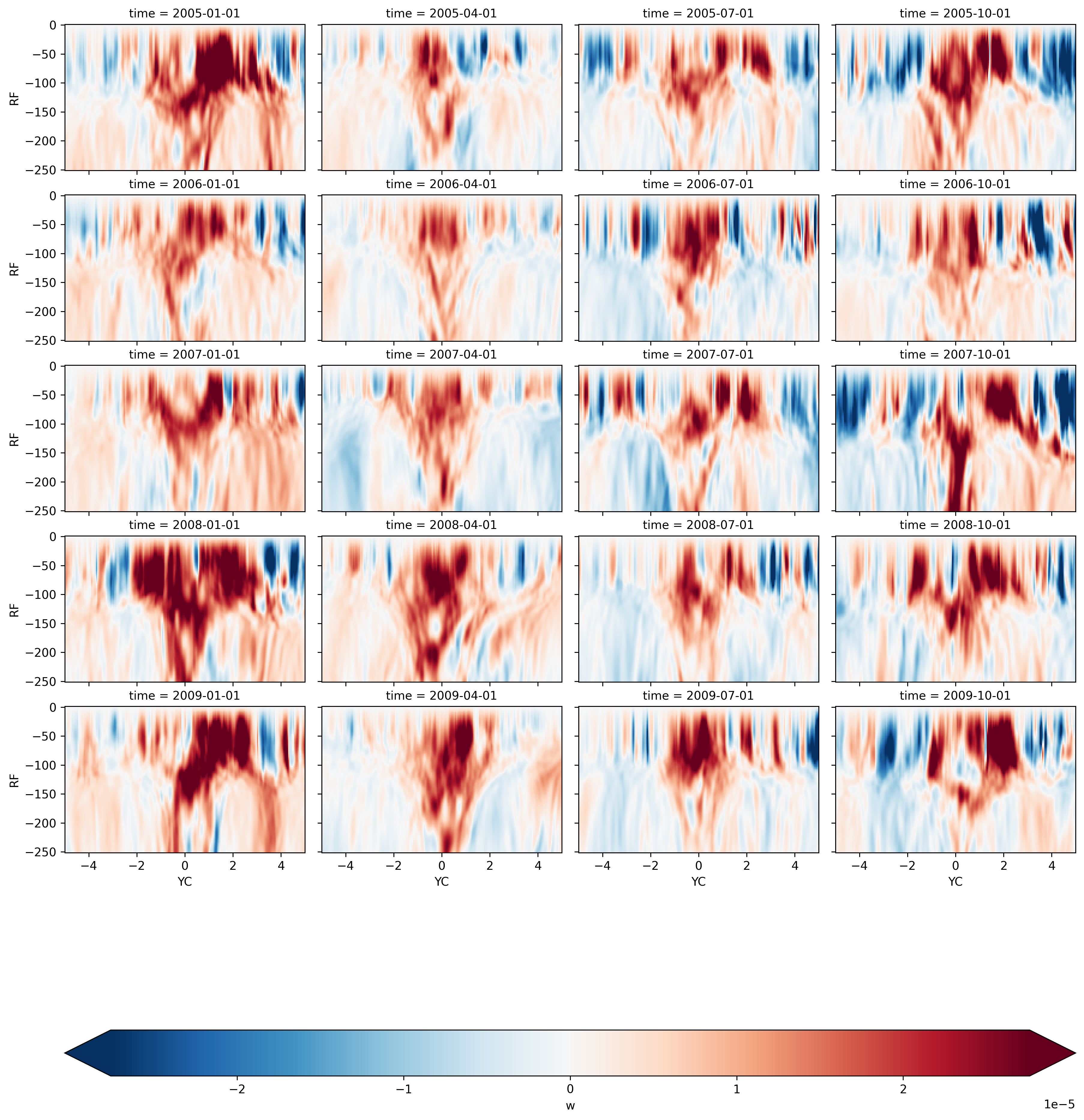
Seasonal mean by year#
seasonalmean.sel(time=slice("2005", "2009")).sel(XC=-140, method="nearest").sel(
YC=slice(-5, 5), RF=slice(-250)
).w.plot(
col="time",
col_wrap=4,
y="RF",
x="YC",
robust=True,
cmap="RdBu_r",
cbar_kwargs={"orientation": "horizontal"},
)
<xarray.plot.facetgrid.FacetGrid at 0x2ba17b6cb2b0>
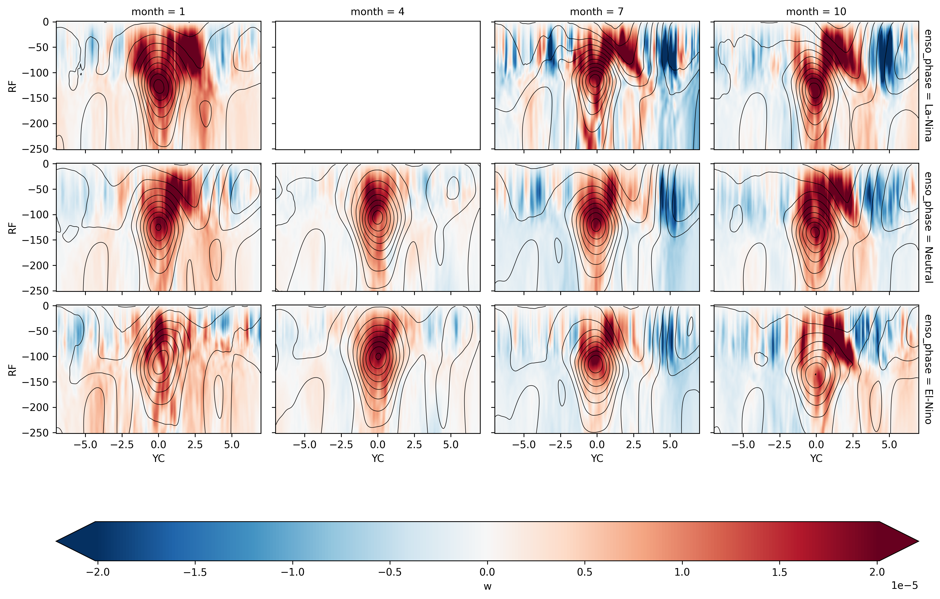
Seasonal mean by ENSO phase#
TODO I am picking the enso phase in the first month of the season. I could do this in a better way…
Show code cell content
enso_phase = pump.obs.make_enso_mask()
seasonalmean.coords["enso_phase"] = (
enso_phase.resample(time="QS").first().reindex(time=seasonalmean.time)
)
Show code cell content
import dask_groupby.xarray
seasonal_phase_mean = dask_groupby.xarray.xarray_reduce(
seasonalmean.sel(XC=[-140], XG=[-140], method="nearest"),
seasonalmean.time.dt.month,
seasonalmean.enso_phase,
func="mean",
fill_value=np.nan,
)
Show code cell content
seasonal_phase_mean.load()
<xarray.Dataset>
Dimensions: (YC: 400, RC: 136, XC: 1, month: 4, enso_phase: 3, XG: 1, RF: 136)
Coordinates:
* RC (RC) float64 -1.25 -3.75 -6.25 -8.75 ... -824.4 -881.7 -944.4
* XC (XC) float64 -140.0
* XG (XG) float64 -140.0
* YC (YC) float64 -9.975 -9.925 -9.875 -9.825 ... 9.875 9.925 9.975
* RF (RF) float64 0.0 -2.5 -5.0 -7.5 ... -747.1 -797.0 -851.7 -911.6
* month (month) int64 1 4 7 10
* enso_phase (enso_phase) object 'La-Nina' 'Neutral' 'El-Nino'
Data variables:
theta (YC, RC, XC, month, enso_phase) float64 27.42 27.86 ... 4.675
u (YC, RC, XG, month, enso_phase) float64 -0.09301 ... -0.01501
w (YC, RF, XC, month, enso_phase) float64 -5.711e-09 ... 7.112e-06
Attributes:
easting: longitude
field_julian_date: 447072
julian_day_unit: days since 1950-01-01 00:00:00
northing: latitude
title: daily snapshot from 1/20 degree Equatorial Pacific MI...- YC: 400
- RC: 136
- XC: 1
- month: 4
- enso_phase: 3
- XG: 1
- RF: 136
- RC(RC)float64-1.25 -3.75 -6.25 ... -881.7 -944.4
- axis :
- Z
array([ -1.25 , -3.75 , -6.25 , -8.75 , -11.25 , -13.75 , -16.25 , -18.75 , -21.25 , -23.75 , -26.25 , -28.75 , -31.25 , -33.75 , -36.25 , -38.75 , -41.25 , -43.75 , -46.25 , -48.75 , -51.25 , -53.75 , -56.25 , -58.75 , -61.25 , -63.75 , -66.25 , -68.75 , -71.25 , -73.75 , -76.25 , -78.75 , -81.25 , -83.75 , -86.25 , -88.75 , -91.25 , -93.75 , -96.25 , -98.75 , -101.25 , -103.75 , -106.25 , -108.75 , -111.25 , -113.75 , -116.25 , -118.75 , -121.25 , -123.75 , -126.25 , -128.75 , -131.25 , -133.75 , -136.25 , -138.75 , -141.25 , -143.75 , -146.25 , -148.75 , -151.25 , -153.75 , -156.25 , -158.75 , -161.25 , -163.75 , -166.25 , -168.75 , -171.25 , -173.75 , -176.25 , -178.75 , -181.25 , -183.75 , -186.25 , -188.75 , -191.25 , -193.75 , -196.25 , -198.75 , -201.25 , -203.75 , -206.25 , -208.75 , -211.25 , -213.75 , -216.25 , -218.75 , -221.25 , -223.75 , -226.25 , -228.75 , -231.25 , -233.75 , -236.25 , -238.75 , -241.25 , -243.75 , -246.25 , -248.75 , -251.368744, -254.236298, -257.376251, -260.814514, -264.579407, -268.701935, -273.216156, -278.15921 , -283.571838, -289.498688, -295.988556, -303.09491 , -310.876404, -319.397156, -328.727356, -338.943939, -350.131165, -362.381104, -375.794739, -390.482697, -406.56604 , -424.177338, -443.4617 , -464.578064, -487.700439, -513.01947 , -540.743774, -571.101929, -604.344116, -640.744324, -680.602478, -724.247192, -772.038147, -824.369263, -881.671814, -944.418091]) - XC(XC)float64-140.0
- axis :
- X
array([-140.])
- XG(XG)float64-140.0
array([-139.975001])
- YC(YC)float64-9.975 -9.925 ... 9.925 9.975
- axis :
- Y
array([-9.975, -9.925, -9.875, ..., 9.875, 9.925, 9.975])
- RF(RF)float640.0 -2.5 -5.0 ... -851.7 -911.6
array([ 0. , -2.5 , -5. , -7.5 , -10. , -12.5 , -15. , -17.5 , -20. , -22.5 , -25. , -27.5 , -30. , -32.5 , -35. , -37.5 , -40. , -42.5 , -45. , -47.5 , -50. , -52.5 , -55. , -57.5 , -60. , -62.5 , -65. , -67.5 , -70. , -72.5 , -75. , -77.5 , -80. , -82.5 , -85. , -87.5 , -90. , -92.5 , -95. , -97.5 , -100. , -102.5 , -105. , -107.5 , -110. , -112.5 , -115. , -117.5 , -120. , -122.5 , -125. , -127.5 , -130. , -132.5 , -135. , -137.5 , -140. , -142.5 , -145. , -147.5 , -150. , -152.5 , -155. , -157.5 , -160. , -162.5 , -165. , -167.5 , -170. , -172.5 , -175. , -177.5 , -180. , -182.5 , -185. , -187.5 , -190. , -192.5 , -195. , -197.5 , -200. , -202.5 , -205. , -207.5 , -210. , -212.5 , -215. , -217.5 , -220. , -222.5 , -225. , -227.5 , -230. , -232.5 , -235. , -237.5 , -240. , -242.5 , -245. , -247.5 , -250. , -252.737503, -255.735107, -259.017395, -262.611603, -266.547211, -270.856689, -275.575592, -280.742798, -286.400909, -292.596497, -299.380615, -306.809204, -314.943604, -323.850708, -333.604004, -344.283905, -355.978394, -368.783813, -382.805695, -398.159698, -414.972412, -433.382294, -453.541107, -475.61499 , -499.785889, -526.252991, -555.234497, -586.969299, -621.718872, -659.769714, -701.435303, -747.059082, -797.017212, -851.721313, -911.622314]) - month(month)int641 4 7 10
array([ 1, 4, 7, 10])
- enso_phase(enso_phase)object'La-Nina' 'Neutral' 'El-Nino'
array(['La-Nina', 'Neutral', 'El-Nino'], dtype=object)
- theta(YC, RC, XC, month, enso_phase)float6427.42 27.86 28.74 ... 4.619 4.675
array([[[[[27.419192 , 27.8551534 , 28.73880768], [ nan, 27.76539612, 28.19641283], [26.48686981, 26.84729513, 27.14731707], [26.72894592, 27.2277298 , 27.74181938]]], [[[27.40752411, 27.84572686, 28.73081207], [ nan, 27.75893402, 28.188797 ], [26.48877716, 26.84544373, 27.14222499], [26.72242126, 27.21812439, 27.72860336]]], [[[27.39732615, 27.83691406, 28.72327995], [ nan, 27.75347137, 28.18251716], [26.48819542, 26.84219021, 27.13742719], [26.71547852, 27.20933914, 27.7172966 ]]], ..., ... ..., [[[ 5.06878662, 5.09346263, 5.2156744 ], [ nan, 5.14725542, 5.18662601], [ 5.33933735, 5.22959985, 5.33699799], [ 5.22690582, 5.20799017, 5.26520061]]], [[[ 4.78859552, 4.8071306 , 4.92052746], [ nan, 4.85159588, 4.89585325], [ 5.02742815, 4.93812943, 5.03494753], [ 4.94215126, 4.91272402, 4.96936226]]], [[[ 4.50488281, 4.52429877, 4.62709427], [ nan, 4.56172657, 4.60404883], [ 4.71506071, 4.64573627, 4.73014559], [ 4.65715637, 4.61946964, 4.67530298]]]]]) - u(YC, RC, XG, month, enso_phase)float64-0.09301 -0.1056 ... -0.01501
array([[[[[-0.09301004, -0.10564631, -0.07485515], [ nan, -0.10385358, -0.11309249], [-0.10117952, -0.1172621 , -0.0873586 ], [-0.0975318 , -0.10590007, -0.04735645]]], [[[-0.07312214, -0.08688883, -0.05806623], [ nan, -0.08462512, -0.09492598], [-0.07599347, -0.09556972, -0.06666265], [-0.07724199, -0.08753194, -0.02954304]]], [[[-0.05995165, -0.07472905, -0.04731032], [ nan, -0.07288393, -0.08367841], [-0.06176363, -0.08261096, -0.05419137], [-0.06424195, -0.07562432, -0.01797123]]], ..., ... ..., [[[-0.05416447, -0.02492077, -0.01387989], [ nan, -0.01653453, -0.03741084], [ 0.01977198, -0.01663588, -0.02025855], [-0.04161796, -0.02008634, -0.01752177]]], [[[-0.05461635, -0.02468956, -0.01327094], [ nan, -0.0184573 , -0.03657472], [ 0.02129319, -0.0162006 , -0.01841395], [-0.04120487, -0.01806772, -0.01622589]]], [[[-0.05487851, -0.02417951, -0.01266 ], [ nan, -0.02056456, -0.03530318], [ 0.02269332, -0.01607642, -0.01630523], [-0.03994213, -0.01610364, -0.01500522]]]]]) - w(YC, RF, XC, month, enso_phase)float64-5.711e-09 -4.505e-09 ... 7.112e-06
array([[[[[-5.71145264e-09, -4.50491516e-09, 7.40605710e-09], [ nan, -1.25016419e-09, -3.14635074e-09], [ 1.96420574e-10, 2.64080175e-09, 2.97787192e-09], [ 3.35545280e-10, 4.51219639e-09, 4.26679847e-09]]], [[[-5.96773854e-07, 4.23601894e-08, 3.03950202e-07], [ nan, 2.03185863e-07, 4.80927409e-07], [-8.67103381e-07, 2.63679138e-07, 5.50959092e-07], [-4.52563199e-08, 1.05137069e-07, -5.73530201e-07]]], [[[-1.14698742e-06, 1.08859897e-07, 6.22070445e-07], [ nan, 4.05119806e-07, 9.47564735e-07], [-1.68241320e-06, 5.41031871e-07, 1.10779495e-06], [-4.61936907e-08, 2.25490595e-07, -1.12296118e-06]]], ..., ... ..., [[[ 2.49251540e-06, -2.84188981e-06, -9.64338142e-07], [ nan, -3.10966811e-06, -2.73967534e-06], [-1.88544607e-06, -2.36282964e-06, 1.99560951e-06], [ 8.41060901e-06, 6.22040125e-06, 7.44746194e-06]]], [[[ 2.59759418e-06, -2.73137893e-06, -8.61151875e-07], [ nan, -3.05679691e-06, -2.80661920e-06], [-1.55325358e-06, -2.47929125e-06, 2.12873445e-06], [ 8.16603424e-06, 6.04666911e-06, 7.27718907e-06]]], [[[ 2.74004014e-06, -2.56421966e-06, -6.61512445e-07], [ nan, -2.93410562e-06, -3.01725393e-06], [-1.34761194e-06, -2.57774708e-06, 2.06139599e-06], [ 8.08279001e-06, 6.08919481e-06, 7.11155099e-06]]]]])
- easting :
- longitude
- field_julian_date :
- 447072
- julian_day_unit :
- days since 1950-01-01 00:00:00
- northing :
- latitude
- title :
- daily snapshot from 1/20 degree Equatorial Pacific MITgcm simulation
There is definitely a northward “bias” in upwelling
The split is more obvious in La-Nina JFM, OND seasons?
Show code cell source
fg = (
seasonal_phase_mean.sel(YC=slice(-7, 7), RF=slice(-250))
.sel(XC=-140, method="nearest")
.w.plot(
col="month",
row="enso_phase",
y="RF",
x="YC",
robust=True,
cmap="RdBu_r",
cbar_kwargs={"orientation": "horizontal"},
)
)
fg.data = (
seasonal_phase_mean.sel(YC=slice(-7, 7), RF=slice(-250))
.sel(XG=-140, method="nearest")
.u
)
fg.map_dataarray(
xr.plot.contour,
y="RC",
x="YC",
levels=21,
colors="k",
linewidths=0.5,
add_colorbar=False,
)
<xarray.plot.facetgrid.FacetGrid at 0x2ba17b4b29a0>
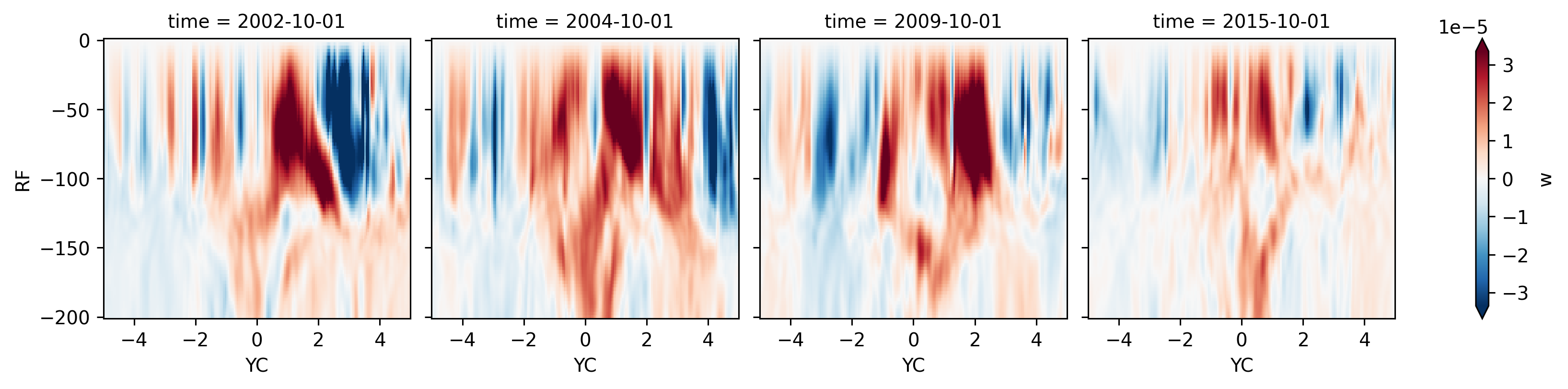
Lets check the OND season for El-Nino years
seasonalmean.sel(XC=-140, method="nearest").sel(
time=seasonalmean.time.dt.month == 10
).query(time="enso_phase == 'El-Nino'").w.sel(RF=slice(-200), YC=slice(-5, 5)).plot(
col="time",
y="RF",
x="YC",
robust=True,
cmap="RdBu_r",
cbar_kwargs={"orientation": "vertical"},
)
<xarray.plot.facetgrid.FacetGrid at 0x2ba182b72fd0>
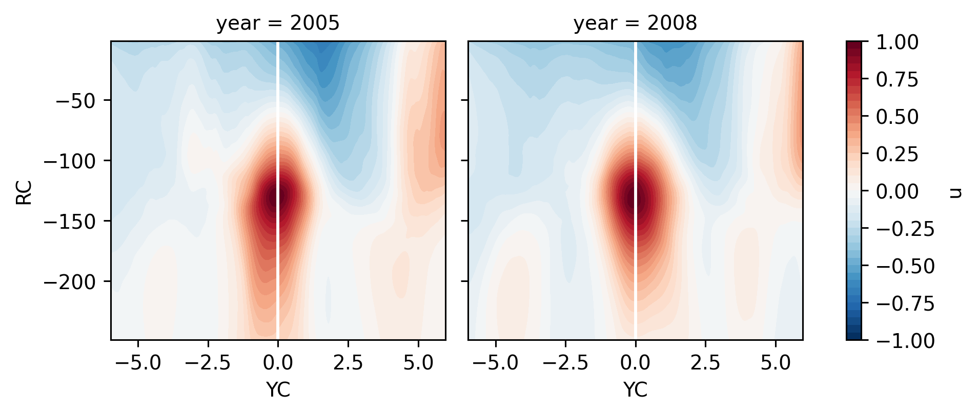
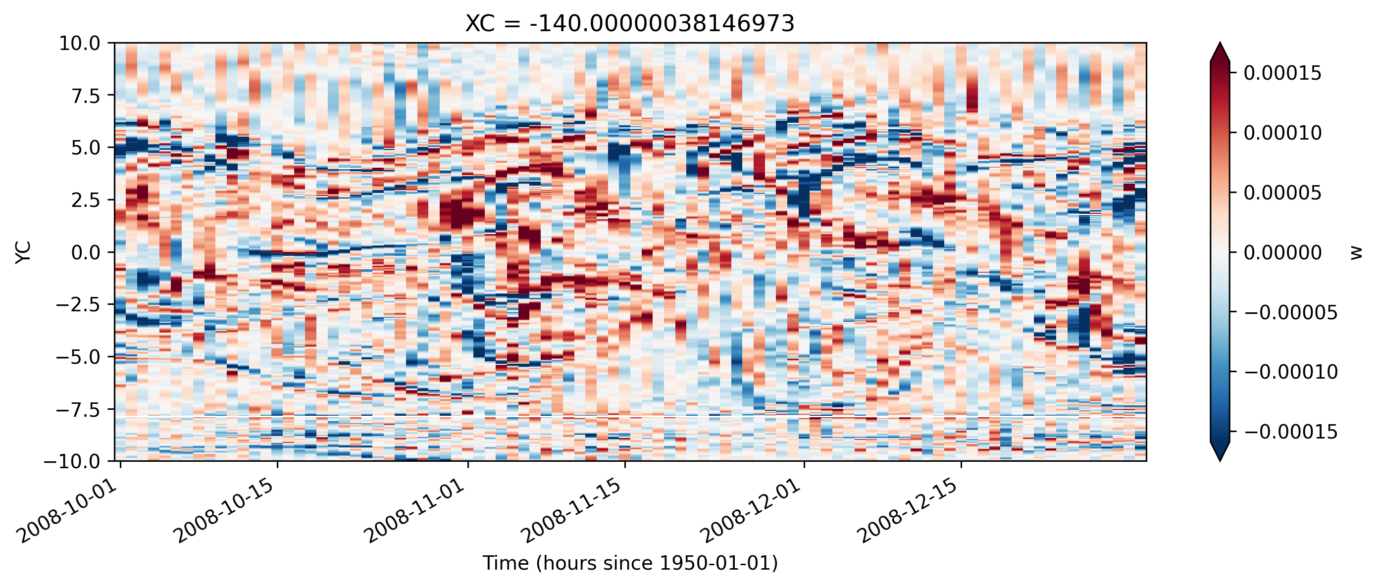
2005 vs 2008 OND at 140W#
2008 has a more pronounced downwelling signal at the equator unlike 2005. But turns out they both have a bunch of TIWs
TODO extend this for 2005, 2006, 2007, 2008.
read data#
Show code cell content
ond05, metrics, grid = pump.model.read_mitgcm_20_year(
state=True,
start="2005-10-01",
stop="2005-12-31", # chunks={"RC": 10, "RF": 10},
)
ond05
2466 2557
<xarray.Dataset>
Dimensions: (RF: 136, YG: 400, XG: 1420, YC: 400, XC: 1420, time: 92, RC: 136)
Coordinates:
* RF (RF) float64 0.0 -2.5 -5.0 -7.5 ... -797.0 -851.7 -911.6
* YG (YG) float64 -10.0 -9.95 -9.9 -9.85 ... 9.8 9.85 9.9 9.95
* XG (XG) float64 -168.0 -168.0 -167.9 ... -97.18 -97.12 -97.08
* YC (YC) float64 -9.975 -9.925 -9.875 ... 9.875 9.925 9.975
* XC (XC) float64 -168.0 -167.9 -167.9 ... -97.15 -97.1 -97.05
* time (time) datetime64[ns] 2005-10-01 2005-10-02 ... 2005-12-31
* RC (RC) float64 -1.25 -3.75 -6.25 ... -824.4 -881.7 -944.4
Data variables: (12/13)
theta (time, RC, YC, XC) float32 dask.array<chunksize=(1, 136, 400, 500), meta=np.ndarray>
u (time, RC, YC, XG) float32 dask.array<chunksize=(1, 136, 400, 500), meta=np.ndarray>
v (time, RC, YG, XC) float32 dask.array<chunksize=(1, 136, 400, 500), meta=np.ndarray>
w (time, RF, YC, XC) float32 dask.array<chunksize=(1, 136, 400, 500), meta=np.ndarray>
salt (time, RC, YC, XC) float32 dask.array<chunksize=(1, 136, 400, 500), meta=np.ndarray>
KPP_diffusivity (time, RF, YC, XC) float32 dask.array<chunksize=(1, 136, 400, 500), meta=np.ndarray>
... ...
N2 (time, RF, YC, XC) float32 dask.array<chunksize=(1, 1, 400, 500), meta=np.ndarray>
S2 (time, RF, YC, XC) float32 dask.array<chunksize=(1, 1, 399, 499), meta=np.ndarray>
Ri (time, RF, YC, XC) float32 dask.array<chunksize=(1, 1, 399, 499), meta=np.ndarray>
mld (time, YC, XC) float64 dask.array<chunksize=(1, 400, 500), meta=np.ndarray>
dcl_base (time, YC, XC) float64 dask.array<chunksize=(1, 399, 499), meta=np.ndarray>
dcl (time, YC, XC) float64 dask.array<chunksize=(1, 399, 499), meta=np.ndarray>
Attributes:
title: daily snapshot from 1/20 degree Equatorial Pacific MI...
easting: longitude
northing: latitude
field_julian_date: 488688
julian_day_unit: days since 1950-01-01 00:00:00- RF: 136
- YG: 400
- XG: 1420
- YC: 400
- XC: 1420
- time: 92
- RC: 136
- RF(RF)float640.0 -2.5 -5.0 ... -851.7 -911.6
- axis :
- Z
- c_grid_axis_shift :
- -0.5
array([ 0. , -2.5 , -5. , -7.5 , -10. , -12.5 , -15. , -17.5 , -20. , -22.5 , -25. , -27.5 , -30. , -32.5 , -35. , -37.5 , -40. , -42.5 , -45. , -47.5 , -50. , -52.5 , -55. , -57.5 , -60. , -62.5 , -65. , -67.5 , -70. , -72.5 , -75. , -77.5 , -80. , -82.5 , -85. , -87.5 , -90. , -92.5 , -95. , -97.5 , -100. , -102.5 , -105. , -107.5 , -110. , -112.5 , -115. , -117.5 , -120. , -122.5 , -125. , -127.5 , -130. , -132.5 , -135. , -137.5 , -140. , -142.5 , -145. , -147.5 , -150. , -152.5 , -155. , -157.5 , -160. , -162.5 , -165. , -167.5 , -170. , -172.5 , -175. , -177.5 , -180. , -182.5 , -185. , -187.5 , -190. , -192.5 , -195. , -197.5 , -200. , -202.5 , -205. , -207.5 , -210. , -212.5 , -215. , -217.5 , -220. , -222.5 , -225. , -227.5 , -230. , -232.5 , -235. , -237.5 , -240. , -242.5 , -245. , -247.5 , -250. , -252.737503, -255.735107, -259.017395, -262.611603, -266.547211, -270.856689, -275.575592, -280.742798, -286.400909, -292.596497, -299.380615, -306.809204, -314.943604, -323.850708, -333.604004, -344.283905, -355.978394, -368.783813, -382.805695, -398.159698, -414.972412, -433.382294, -453.541107, -475.61499 , -499.785889, -526.252991, -555.234497, -586.969299, -621.718872, -659.769714, -701.435303, -747.059082, -797.017212, -851.721313, -911.622314]) - YG(YG)float64-10.0 -9.95 -9.9 ... 9.85 9.9 9.95
- axis :
- Y
array([-10. , -9.95, -9.9 , ..., 9.85, 9.9 , 9.95])
- XG(XG)float64-168.0 -168.0 ... -97.12 -97.08
- axis :
- X
array([-168.025 , -167.975 , -167.925 , ..., -97.175002, -97.124998, -97.075003]) - YC(YC)float64-9.975 -9.925 ... 9.925 9.975
- axis :
- Y
array([-9.975, -9.925, -9.875, ..., 9.875, 9.925, 9.975])
- XC(XC)float64-168.0 -167.9 ... -97.1 -97.05
- axis :
- X
array([-168. , -167.95 , -167.9 , ..., -97.15 , -97.099997, -97.050002]) - time(time)datetime64[ns]2005-10-01 ... 2005-12-31
- long_name :
- Time (hours since 1950-01-01)
- standard_name :
- time
- axis :
- T
- _CoordinateAxisType :
- Time
array(['2005-10-01T00:00:00.000000000', '2005-10-02T00:00:00.000000000', '2005-10-03T00:00:00.000000000', '2005-10-04T00:00:00.000000000', '2005-10-05T00:00:00.000000000', '2005-10-06T00:00:00.000000000', '2005-10-07T00:00:00.000000000', '2005-10-08T00:00:00.000000000', '2005-10-09T00:00:00.000000000', '2005-10-10T00:00:00.000000000', '2005-10-11T00:00:00.000000000', '2005-10-12T00:00:00.000000000', '2005-10-13T00:00:00.000000000', '2005-10-14T00:00:00.000000000', '2005-10-15T00:00:00.000000000', '2005-10-16T00:00:00.000000000', '2005-10-17T00:00:00.000000000', '2005-10-18T00:00:00.000000000', '2005-10-19T00:00:00.000000000', '2005-10-20T00:00:00.000000000', '2005-10-21T00:00:00.000000000', '2005-10-22T00:00:00.000000000', '2005-10-23T00:00:00.000000000', '2005-10-24T00:00:00.000000000', '2005-10-25T00:00:00.000000000', '2005-10-26T00:00:00.000000000', '2005-10-27T00:00:00.000000000', '2005-10-28T00:00:00.000000000', '2005-10-29T00:00:00.000000000', '2005-10-30T00:00:00.000000000', '2005-10-31T00:00:00.000000000', '2005-11-01T00:00:00.000000000', '2005-11-02T00:00:00.000000000', '2005-11-03T00:00:00.000000000', '2005-11-04T00:00:00.000000000', '2005-11-05T00:00:00.000000000', '2005-11-06T00:00:00.000000000', '2005-11-07T00:00:00.000000000', '2005-11-08T00:00:00.000000000', '2005-11-09T00:00:00.000000000', '2005-11-10T00:00:00.000000000', '2005-11-11T00:00:00.000000000', '2005-11-12T00:00:00.000000000', '2005-11-13T00:00:00.000000000', '2005-11-14T00:00:00.000000000', '2005-11-15T00:00:00.000000000', '2005-11-16T00:00:00.000000000', '2005-11-17T00:00:00.000000000', '2005-11-18T00:00:00.000000000', '2005-11-19T00:00:00.000000000', '2005-11-20T00:00:00.000000000', '2005-11-21T00:00:00.000000000', '2005-11-22T00:00:00.000000000', '2005-11-23T00:00:00.000000000', '2005-11-24T00:00:00.000000000', '2005-11-25T00:00:00.000000000', '2005-11-26T00:00:00.000000000', '2005-11-27T00:00:00.000000000', '2005-11-28T00:00:00.000000000', '2005-11-29T00:00:00.000000000', '2005-11-30T00:00:00.000000000', '2005-12-01T00:00:00.000000000', '2005-12-02T00:00:00.000000000', '2005-12-03T00:00:00.000000000', '2005-12-04T00:00:00.000000000', '2005-12-05T00:00:00.000000000', '2005-12-06T00:00:00.000000000', '2005-12-07T00:00:00.000000000', '2005-12-08T00:00:00.000000000', '2005-12-09T00:00:00.000000000', '2005-12-10T00:00:00.000000000', '2005-12-11T00:00:00.000000000', '2005-12-12T00:00:00.000000000', '2005-12-13T00:00:00.000000000', '2005-12-14T00:00:00.000000000', '2005-12-15T00:00:00.000000000', '2005-12-16T00:00:00.000000000', '2005-12-17T00:00:00.000000000', '2005-12-18T00:00:00.000000000', '2005-12-19T00:00:00.000000000', '2005-12-20T00:00:00.000000000', '2005-12-21T00:00:00.000000000', '2005-12-22T00:00:00.000000000', '2005-12-23T00:00:00.000000000', '2005-12-24T00:00:00.000000000', '2005-12-25T00:00:00.000000000', '2005-12-26T00:00:00.000000000', '2005-12-27T00:00:00.000000000', '2005-12-28T00:00:00.000000000', '2005-12-29T00:00:00.000000000', '2005-12-30T00:00:00.000000000', '2005-12-31T00:00:00.000000000'], dtype='datetime64[ns]') - RC(RC)float64-1.25 -3.75 -6.25 ... -881.7 -944.4
- axis :
- Z
array([ -1.25 , -3.75 , -6.25 , -8.75 , -11.25 , -13.75 , -16.25 , -18.75 , -21.25 , -23.75 , -26.25 , -28.75 , -31.25 , -33.75 , -36.25 , -38.75 , -41.25 , -43.75 , -46.25 , -48.75 , -51.25 , -53.75 , -56.25 , -58.75 , -61.25 , -63.75 , -66.25 , -68.75 , -71.25 , -73.75 , -76.25 , -78.75 , -81.25 , -83.75 , -86.25 , -88.75 , -91.25 , -93.75 , -96.25 , -98.75 , -101.25 , -103.75 , -106.25 , -108.75 , -111.25 , -113.75 , -116.25 , -118.75 , -121.25 , -123.75 , -126.25 , -128.75 , -131.25 , -133.75 , -136.25 , -138.75 , -141.25 , -143.75 , -146.25 , -148.75 , -151.25 , -153.75 , -156.25 , -158.75 , -161.25 , -163.75 , -166.25 , -168.75 , -171.25 , -173.75 , -176.25 , -178.75 , -181.25 , -183.75 , -186.25 , -188.75 , -191.25 , -193.75 , -196.25 , -198.75 , -201.25 , -203.75 , -206.25 , -208.75 , -211.25 , -213.75 , -216.25 , -218.75 , -221.25 , -223.75 , -226.25 , -228.75 , -231.25 , -233.75 , -236.25 , -238.75 , -241.25 , -243.75 , -246.25 , -248.75 , -251.368744, -254.236298, -257.376251, -260.814514, -264.579407, -268.701935, -273.216156, -278.15921 , -283.571838, -289.498688, -295.988556, -303.09491 , -310.876404, -319.397156, -328.727356, -338.943939, -350.131165, -362.381104, -375.794739, -390.482697, -406.56604 , -424.177338, -443.4617 , -464.578064, -487.700439, -513.01947 , -540.743774, -571.101929, -604.344116, -640.744324, -680.602478, -724.247192, -772.038147, -824.369263, -881.671814, -944.418091])
- theta(time, RC, YC, XC)float32dask.array<chunksize=(1, 136, 400, 500), meta=np.ndarray>
Array Chunk Bytes 26.47 GiB 103.76 MiB Shape (92, 136, 400, 1420) (1, 136, 400, 500) Count 644 Tasks 276 Chunks Type float32 numpy.ndarray - u(time, RC, YC, XG)float32dask.array<chunksize=(1, 136, 400, 500), meta=np.ndarray>
Array Chunk Bytes 26.47 GiB 103.76 MiB Shape (92, 136, 400, 1420) (1, 136, 400, 500) Count 644 Tasks 276 Chunks Type float32 numpy.ndarray - v(time, RC, YG, XC)float32dask.array<chunksize=(1, 136, 400, 500), meta=np.ndarray>
Array Chunk Bytes 26.47 GiB 103.76 MiB Shape (92, 136, 400, 1420) (1, 136, 400, 500) Count 644 Tasks 276 Chunks Type float32 numpy.ndarray - w(time, RF, YC, XC)float32dask.array<chunksize=(1, 136, 400, 500), meta=np.ndarray>
Array Chunk Bytes 26.47 GiB 103.76 MiB Shape (92, 136, 400, 1420) (1, 136, 400, 500) Count 644 Tasks 276 Chunks Type float32 numpy.ndarray - salt(time, RC, YC, XC)float32dask.array<chunksize=(1, 136, 400, 500), meta=np.ndarray>
Array Chunk Bytes 26.47 GiB 103.76 MiB Shape (92, 136, 400, 1420) (1, 136, 400, 500) Count 644 Tasks 276 Chunks Type float32 numpy.ndarray - KPP_diffusivity(time, RF, YC, XC)float32dask.array<chunksize=(1, 136, 400, 500), meta=np.ndarray>
Array Chunk Bytes 26.47 GiB 103.76 MiB Shape (92, 136, 400, 1420) (1, 136, 400, 500) Count 644 Tasks 276 Chunks Type float32 numpy.ndarray - dens(time, RC, YC, XC)float32dask.array<chunksize=(1, 136, 400, 500), meta=np.ndarray>
Array Chunk Bytes 26.47 GiB 103.76 MiB Shape (92, 136, 400, 1420) (1, 136, 400, 500) Count 1841 Tasks 276 Chunks Type float32 numpy.ndarray - N2(time, RF, YC, XC)float32dask.array<chunksize=(1, 1, 400, 500), meta=np.ndarray>
Array Chunk Bytes 26.47 GiB 103.00 MiB Shape (92, 136, 400, 1420) (1, 135, 400, 500) Count 4606 Tasks 552 Chunks Type float32 numpy.ndarray - S2(time, RF, YC, XC)float32dask.array<chunksize=(1, 1, 399, 499), meta=np.ndarray>
Array Chunk Bytes 26.47 GiB 102.53 MiB Shape (92, 136, 400, 1420) (1, 135, 399, 499) Count 29629 Tasks 2208 Chunks Type float32 numpy.ndarray - Ri(time, RF, YC, XC)float32dask.array<chunksize=(1, 1, 399, 499), meta=np.ndarray>
Array Chunk Bytes 26.47 GiB 102.53 MiB Shape (92, 136, 400, 1420) (1, 135, 399, 499) Count 40854 Tasks 2208 Chunks Type float32 numpy.ndarray - mld(time, YC, XC)float64dask.array<chunksize=(1, 400, 500), meta=np.ndarray>
- long_name :
- MLD
- units :
- m
- description :
- Interpolate density to 1m grid. Search for max depth where |drho| > 0.015 and N2 > 1e-05
Array Chunk Bytes 398.68 MiB 1.53 MiB Shape (92, 400, 1420) (1, 400, 500) Count 6810 Tasks 276 Chunks Type float64 numpy.ndarray - dcl_base(time, YC, XC)float64dask.array<chunksize=(1, 399, 499), meta=np.ndarray>
- long_name :
- $z_{Ri}$
- units :
- m
- description :
- Interpolate density to 1m grid. Search for max depth where |drho| > 0.015 and N2 > 1e-05
Array Chunk Bytes 398.68 MiB 1.52 MiB Shape (92, 400, 1420) (1, 399, 499) Count 59808 Tasks 1104 Chunks Type float64 numpy.ndarray - dcl(time, YC, XC)float64dask.array<chunksize=(1, 399, 499), meta=np.ndarray>
- long_name :
- DCL
- units :
- m
- description :
- Interpolate density to 1m grid. Search for max depth where |drho| > 0.015 and N2 > 1e-05
Array Chunk Bytes 398.68 MiB 1.52 MiB Shape (92, 400, 1420) (1, 399, 499) Count 60912 Tasks 1104 Chunks Type float64 numpy.ndarray
- title :
- daily snapshot from 1/20 degree Equatorial Pacific MITgcm simulation
- easting :
- longitude
- northing :
- latitude
- field_julian_date :
- 488688
- julian_day_unit :
- days since 1950-01-01 00:00:00
Show code cell content
ond08, metrics, grid = pump.model.read_mitgcm_20_year(
state=True,
start="2008-10-01",
stop="2008-12-31", # chunks={"RC": 10, "RF": 10},
)
ond08
3562 3653
<xarray.Dataset>
Dimensions: (RF: 136, YG: 400, XG: 1420, YC: 400, XC: 1420, time: 92, RC: 136)
Coordinates:
* RF (RF) float64 0.0 -2.5 -5.0 -7.5 ... -797.0 -851.7 -911.6
* YG (YG) float64 -10.0 -9.95 -9.9 -9.85 ... 9.8 9.85 9.9 9.95
* XG (XG) float64 -168.0 -168.0 -167.9 ... -97.18 -97.12 -97.08
* YC (YC) float64 -9.975 -9.925 -9.875 ... 9.875 9.925 9.975
* XC (XC) float64 -168.0 -167.9 -167.9 ... -97.15 -97.1 -97.05
* time (time) datetime64[ns] 2008-10-01 2008-10-02 ... 2008-12-31
* RC (RC) float64 -1.25 -3.75 -6.25 ... -824.4 -881.7 -944.4
Data variables: (12/13)
theta (time, RC, YC, XC) float32 dask.array<chunksize=(1, 136, 400, 500), meta=np.ndarray>
u (time, RC, YC, XG) float32 dask.array<chunksize=(1, 136, 400, 500), meta=np.ndarray>
v (time, RC, YG, XC) float32 dask.array<chunksize=(1, 136, 400, 500), meta=np.ndarray>
w (time, RF, YC, XC) float32 dask.array<chunksize=(1, 136, 400, 500), meta=np.ndarray>
salt (time, RC, YC, XC) float32 dask.array<chunksize=(1, 136, 400, 500), meta=np.ndarray>
KPP_diffusivity (time, RF, YC, XC) float32 dask.array<chunksize=(1, 136, 400, 500), meta=np.ndarray>
... ...
N2 (time, RF, YC, XC) float32 dask.array<chunksize=(1, 1, 400, 500), meta=np.ndarray>
S2 (time, RF, YC, XC) float32 dask.array<chunksize=(1, 1, 399, 499), meta=np.ndarray>
Ri (time, RF, YC, XC) float32 dask.array<chunksize=(1, 1, 399, 499), meta=np.ndarray>
mld (time, YC, XC) float64 dask.array<chunksize=(1, 400, 500), meta=np.ndarray>
dcl_base (time, YC, XC) float64 dask.array<chunksize=(1, 399, 499), meta=np.ndarray>
dcl (time, YC, XC) float64 dask.array<chunksize=(1, 399, 499), meta=np.ndarray>
Attributes:
title: daily snapshot from 1/20 degree Equatorial Pacific MI...
easting: longitude
northing: latitude
field_julian_date: 514992
julian_day_unit: days since 1950-01-01 00:00:00- RF: 136
- YG: 400
- XG: 1420
- YC: 400
- XC: 1420
- time: 92
- RC: 136
- RF(RF)float640.0 -2.5 -5.0 ... -851.7 -911.6
- axis :
- Z
- c_grid_axis_shift :
- -0.5
array([ 0. , -2.5 , -5. , -7.5 , -10. , -12.5 , -15. , -17.5 , -20. , -22.5 , -25. , -27.5 , -30. , -32.5 , -35. , -37.5 , -40. , -42.5 , -45. , -47.5 , -50. , -52.5 , -55. , -57.5 , -60. , -62.5 , -65. , -67.5 , -70. , -72.5 , -75. , -77.5 , -80. , -82.5 , -85. , -87.5 , -90. , -92.5 , -95. , -97.5 , -100. , -102.5 , -105. , -107.5 , -110. , -112.5 , -115. , -117.5 , -120. , -122.5 , -125. , -127.5 , -130. , -132.5 , -135. , -137.5 , -140. , -142.5 , -145. , -147.5 , -150. , -152.5 , -155. , -157.5 , -160. , -162.5 , -165. , -167.5 , -170. , -172.5 , -175. , -177.5 , -180. , -182.5 , -185. , -187.5 , -190. , -192.5 , -195. , -197.5 , -200. , -202.5 , -205. , -207.5 , -210. , -212.5 , -215. , -217.5 , -220. , -222.5 , -225. , -227.5 , -230. , -232.5 , -235. , -237.5 , -240. , -242.5 , -245. , -247.5 , -250. , -252.737503, -255.735107, -259.017395, -262.611603, -266.547211, -270.856689, -275.575592, -280.742798, -286.400909, -292.596497, -299.380615, -306.809204, -314.943604, -323.850708, -333.604004, -344.283905, -355.978394, -368.783813, -382.805695, -398.159698, -414.972412, -433.382294, -453.541107, -475.61499 , -499.785889, -526.252991, -555.234497, -586.969299, -621.718872, -659.769714, -701.435303, -747.059082, -797.017212, -851.721313, -911.622314]) - YG(YG)float64-10.0 -9.95 -9.9 ... 9.85 9.9 9.95
- axis :
- Y
array([-10. , -9.95, -9.9 , ..., 9.85, 9.9 , 9.95])
- XG(XG)float64-168.0 -168.0 ... -97.12 -97.08
- axis :
- X
array([-168.025 , -167.975 , -167.925 , ..., -97.175002, -97.124998, -97.075003]) - YC(YC)float64-9.975 -9.925 ... 9.925 9.975
- axis :
- Y
array([-9.975, -9.925, -9.875, ..., 9.875, 9.925, 9.975])
- XC(XC)float64-168.0 -167.9 ... -97.1 -97.05
- axis :
- X
array([-168. , -167.95 , -167.9 , ..., -97.15 , -97.099997, -97.050002]) - time(time)datetime64[ns]2008-10-01 ... 2008-12-31
- long_name :
- Time (hours since 1950-01-01)
- standard_name :
- time
- axis :
- T
- _CoordinateAxisType :
- Time
array(['2008-10-01T00:00:00.000000000', '2008-10-02T00:00:00.000000000', '2008-10-03T00:00:00.000000000', '2008-10-04T00:00:00.000000000', '2008-10-05T00:00:00.000000000', '2008-10-06T00:00:00.000000000', '2008-10-07T00:00:00.000000000', '2008-10-08T00:00:00.000000000', '2008-10-09T00:00:00.000000000', '2008-10-10T00:00:00.000000000', '2008-10-11T00:00:00.000000000', '2008-10-12T00:00:00.000000000', '2008-10-13T00:00:00.000000000', '2008-10-14T00:00:00.000000000', '2008-10-15T00:00:00.000000000', '2008-10-16T00:00:00.000000000', '2008-10-17T00:00:00.000000000', '2008-10-18T00:00:00.000000000', '2008-10-19T00:00:00.000000000', '2008-10-20T00:00:00.000000000', '2008-10-21T00:00:00.000000000', '2008-10-22T00:00:00.000000000', '2008-10-23T00:00:00.000000000', '2008-10-24T00:00:00.000000000', '2008-10-25T00:00:00.000000000', '2008-10-26T00:00:00.000000000', '2008-10-27T00:00:00.000000000', '2008-10-28T00:00:00.000000000', '2008-10-29T00:00:00.000000000', '2008-10-30T00:00:00.000000000', '2008-10-31T00:00:00.000000000', '2008-11-01T00:00:00.000000000', '2008-11-02T00:00:00.000000000', '2008-11-03T00:00:00.000000000', '2008-11-04T00:00:00.000000000', '2008-11-05T00:00:00.000000000', '2008-11-06T00:00:00.000000000', '2008-11-07T00:00:00.000000000', '2008-11-08T00:00:00.000000000', '2008-11-09T00:00:00.000000000', '2008-11-10T00:00:00.000000000', '2008-11-11T00:00:00.000000000', '2008-11-12T00:00:00.000000000', '2008-11-13T00:00:00.000000000', '2008-11-14T00:00:00.000000000', '2008-11-15T00:00:00.000000000', '2008-11-16T00:00:00.000000000', '2008-11-17T00:00:00.000000000', '2008-11-18T00:00:00.000000000', '2008-11-19T00:00:00.000000000', '2008-11-20T00:00:00.000000000', '2008-11-21T00:00:00.000000000', '2008-11-22T00:00:00.000000000', '2008-11-23T00:00:00.000000000', '2008-11-24T00:00:00.000000000', '2008-11-25T00:00:00.000000000', '2008-11-26T00:00:00.000000000', '2008-11-27T00:00:00.000000000', '2008-11-28T00:00:00.000000000', '2008-11-29T00:00:00.000000000', '2008-11-30T00:00:00.000000000', '2008-12-01T00:00:00.000000000', '2008-12-02T00:00:00.000000000', '2008-12-03T00:00:00.000000000', '2008-12-04T00:00:00.000000000', '2008-12-05T00:00:00.000000000', '2008-12-06T00:00:00.000000000', '2008-12-07T00:00:00.000000000', '2008-12-08T00:00:00.000000000', '2008-12-09T00:00:00.000000000', '2008-12-10T00:00:00.000000000', '2008-12-11T00:00:00.000000000', '2008-12-12T00:00:00.000000000', '2008-12-13T00:00:00.000000000', '2008-12-14T00:00:00.000000000', '2008-12-15T00:00:00.000000000', '2008-12-16T00:00:00.000000000', '2008-12-17T00:00:00.000000000', '2008-12-18T00:00:00.000000000', '2008-12-19T00:00:00.000000000', '2008-12-20T00:00:00.000000000', '2008-12-21T00:00:00.000000000', '2008-12-22T00:00:00.000000000', '2008-12-23T00:00:00.000000000', '2008-12-24T00:00:00.000000000', '2008-12-25T00:00:00.000000000', '2008-12-26T00:00:00.000000000', '2008-12-27T00:00:00.000000000', '2008-12-28T00:00:00.000000000', '2008-12-29T00:00:00.000000000', '2008-12-30T00:00:00.000000000', '2008-12-31T00:00:00.000000000'], dtype='datetime64[ns]') - RC(RC)float64-1.25 -3.75 -6.25 ... -881.7 -944.4
- axis :
- Z
array([ -1.25 , -3.75 , -6.25 , -8.75 , -11.25 , -13.75 , -16.25 , -18.75 , -21.25 , -23.75 , -26.25 , -28.75 , -31.25 , -33.75 , -36.25 , -38.75 , -41.25 , -43.75 , -46.25 , -48.75 , -51.25 , -53.75 , -56.25 , -58.75 , -61.25 , -63.75 , -66.25 , -68.75 , -71.25 , -73.75 , -76.25 , -78.75 , -81.25 , -83.75 , -86.25 , -88.75 , -91.25 , -93.75 , -96.25 , -98.75 , -101.25 , -103.75 , -106.25 , -108.75 , -111.25 , -113.75 , -116.25 , -118.75 , -121.25 , -123.75 , -126.25 , -128.75 , -131.25 , -133.75 , -136.25 , -138.75 , -141.25 , -143.75 , -146.25 , -148.75 , -151.25 , -153.75 , -156.25 , -158.75 , -161.25 , -163.75 , -166.25 , -168.75 , -171.25 , -173.75 , -176.25 , -178.75 , -181.25 , -183.75 , -186.25 , -188.75 , -191.25 , -193.75 , -196.25 , -198.75 , -201.25 , -203.75 , -206.25 , -208.75 , -211.25 , -213.75 , -216.25 , -218.75 , -221.25 , -223.75 , -226.25 , -228.75 , -231.25 , -233.75 , -236.25 , -238.75 , -241.25 , -243.75 , -246.25 , -248.75 , -251.368744, -254.236298, -257.376251, -260.814514, -264.579407, -268.701935, -273.216156, -278.15921 , -283.571838, -289.498688, -295.988556, -303.09491 , -310.876404, -319.397156, -328.727356, -338.943939, -350.131165, -362.381104, -375.794739, -390.482697, -406.56604 , -424.177338, -443.4617 , -464.578064, -487.700439, -513.01947 , -540.743774, -571.101929, -604.344116, -640.744324, -680.602478, -724.247192, -772.038147, -824.369263, -881.671814, -944.418091])
- theta(time, RC, YC, XC)float32dask.array<chunksize=(1, 136, 400, 500), meta=np.ndarray>
Array Chunk Bytes 26.47 GiB 103.76 MiB Shape (92, 136, 400, 1420) (1, 136, 400, 500) Count 644 Tasks 276 Chunks Type float32 numpy.ndarray - u(time, RC, YC, XG)float32dask.array<chunksize=(1, 136, 400, 500), meta=np.ndarray>
Array Chunk Bytes 26.47 GiB 103.76 MiB Shape (92, 136, 400, 1420) (1, 136, 400, 500) Count 644 Tasks 276 Chunks Type float32 numpy.ndarray - v(time, RC, YG, XC)float32dask.array<chunksize=(1, 136, 400, 500), meta=np.ndarray>
Array Chunk Bytes 26.47 GiB 103.76 MiB Shape (92, 136, 400, 1420) (1, 136, 400, 500) Count 644 Tasks 276 Chunks Type float32 numpy.ndarray - w(time, RF, YC, XC)float32dask.array<chunksize=(1, 136, 400, 500), meta=np.ndarray>
Array Chunk Bytes 26.47 GiB 103.76 MiB Shape (92, 136, 400, 1420) (1, 136, 400, 500) Count 644 Tasks 276 Chunks Type float32 numpy.ndarray - salt(time, RC, YC, XC)float32dask.array<chunksize=(1, 136, 400, 500), meta=np.ndarray>
Array Chunk Bytes 26.47 GiB 103.76 MiB Shape (92, 136, 400, 1420) (1, 136, 400, 500) Count 644 Tasks 276 Chunks Type float32 numpy.ndarray - KPP_diffusivity(time, RF, YC, XC)float32dask.array<chunksize=(1, 136, 400, 500), meta=np.ndarray>
Array Chunk Bytes 26.47 GiB 103.76 MiB Shape (92, 136, 400, 1420) (1, 136, 400, 500) Count 644 Tasks 276 Chunks Type float32 numpy.ndarray - dens(time, RC, YC, XC)float32dask.array<chunksize=(1, 136, 400, 500), meta=np.ndarray>
Array Chunk Bytes 26.47 GiB 103.76 MiB Shape (92, 136, 400, 1420) (1, 136, 400, 500) Count 1841 Tasks 276 Chunks Type float32 numpy.ndarray - N2(time, RF, YC, XC)float32dask.array<chunksize=(1, 1, 400, 500), meta=np.ndarray>
Array Chunk Bytes 26.47 GiB 103.00 MiB Shape (92, 136, 400, 1420) (1, 135, 400, 500) Count 4606 Tasks 552 Chunks Type float32 numpy.ndarray - S2(time, RF, YC, XC)float32dask.array<chunksize=(1, 1, 399, 499), meta=np.ndarray>
Array Chunk Bytes 26.47 GiB 102.53 MiB Shape (92, 136, 400, 1420) (1, 135, 399, 499) Count 29629 Tasks 2208 Chunks Type float32 numpy.ndarray - Ri(time, RF, YC, XC)float32dask.array<chunksize=(1, 1, 399, 499), meta=np.ndarray>
Array Chunk Bytes 26.47 GiB 102.53 MiB Shape (92, 136, 400, 1420) (1, 135, 399, 499) Count 40854 Tasks 2208 Chunks Type float32 numpy.ndarray - mld(time, YC, XC)float64dask.array<chunksize=(1, 400, 500), meta=np.ndarray>
- long_name :
- MLD
- units :
- m
- description :
- Interpolate density to 1m grid. Search for max depth where |drho| > 0.015 and N2 > 1e-05
Array Chunk Bytes 398.68 MiB 1.53 MiB Shape (92, 400, 1420) (1, 400, 500) Count 6810 Tasks 276 Chunks Type float64 numpy.ndarray - dcl_base(time, YC, XC)float64dask.array<chunksize=(1, 399, 499), meta=np.ndarray>
- long_name :
- $z_{Ri}$
- units :
- m
- description :
- Interpolate density to 1m grid. Search for max depth where |drho| > 0.015 and N2 > 1e-05
Array Chunk Bytes 398.68 MiB 1.52 MiB Shape (92, 400, 1420) (1, 399, 499) Count 59808 Tasks 1104 Chunks Type float64 numpy.ndarray - dcl(time, YC, XC)float64dask.array<chunksize=(1, 399, 499), meta=np.ndarray>
- long_name :
- DCL
- units :
- m
- description :
- Interpolate density to 1m grid. Search for max depth where |drho| > 0.015 and N2 > 1e-05
Array Chunk Bytes 398.68 MiB 1.52 MiB Shape (92, 400, 1420) (1, 399, 499) Count 60912 Tasks 1104 Chunks Type float64 numpy.ndarray
- title :
- daily snapshot from 1/20 degree Equatorial Pacific MITgcm simulation
- easting :
- longitude
- northing :
- latitude
- field_julian_date :
- 514992
- julian_day_unit :
- days since 1950-01-01 00:00:00
Show code cell content
ond0508 = xr.concat([ond05.drop("time"), ond08.drop("time")], dim="year")
ond0508["year"] = [2005, 2008]
u, v, T#
I am looking for what’s different in 2005 vs 2008.
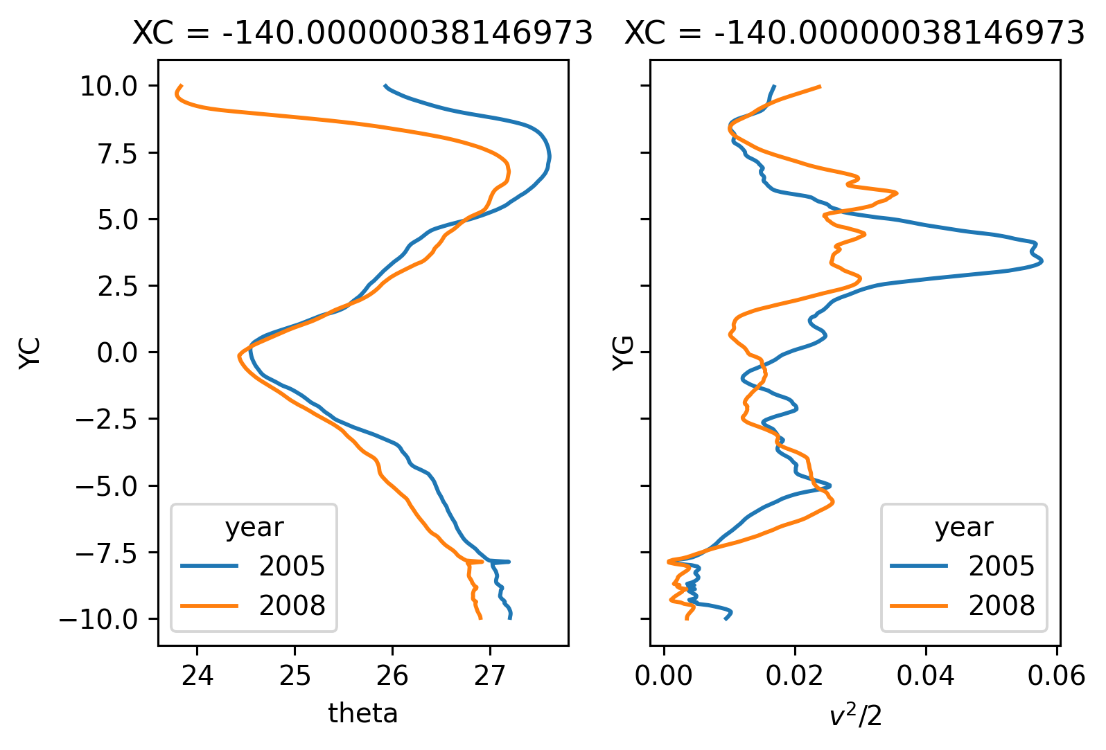
EUC is in basically the same place. similar speed. similar latitude for EUC maximum.
SEC is narrower in 2005 and faster.
Cold tongue using top 100m mean temp is in basically the same place
In 2005, \(v^2\) has a larger northern maximum. This is the largest difference I’ve seen so far
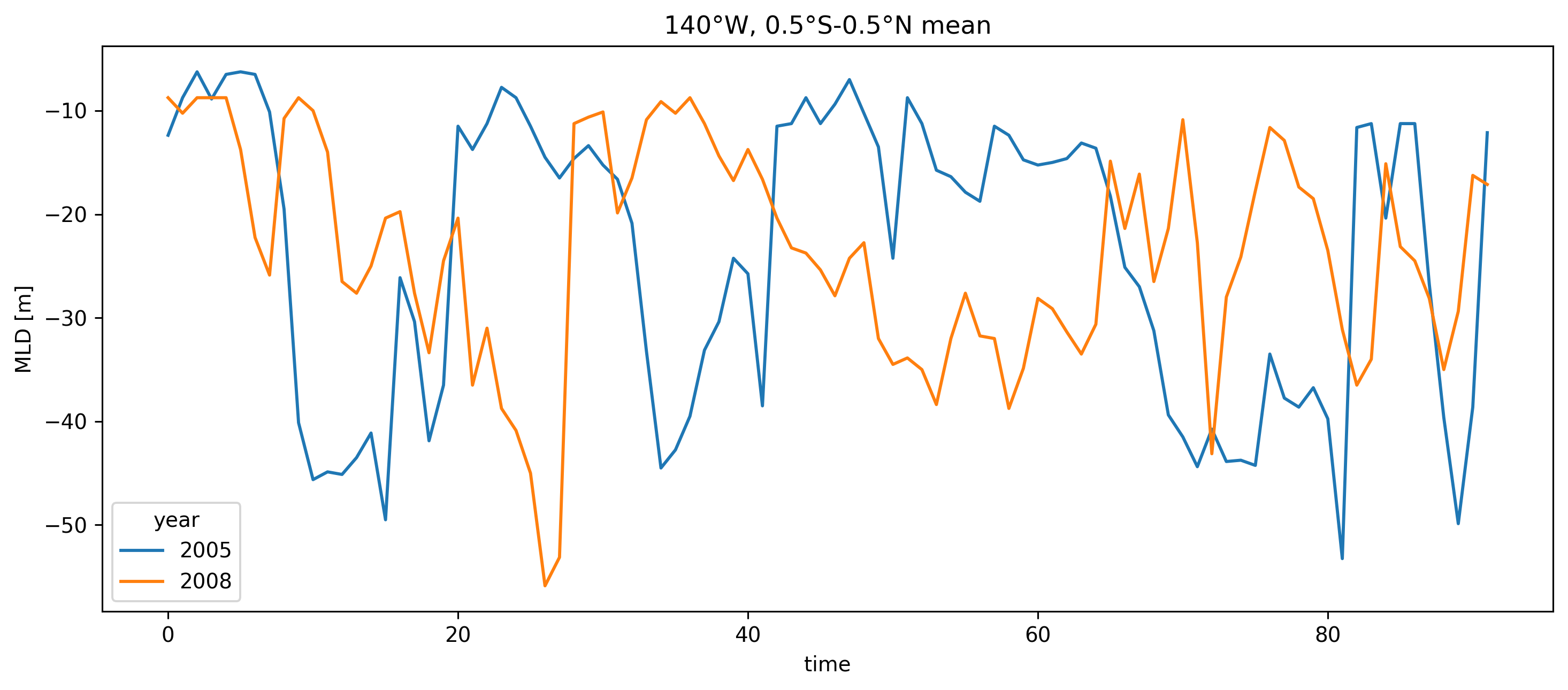
MLD looks similar; deepest is 40m at eq
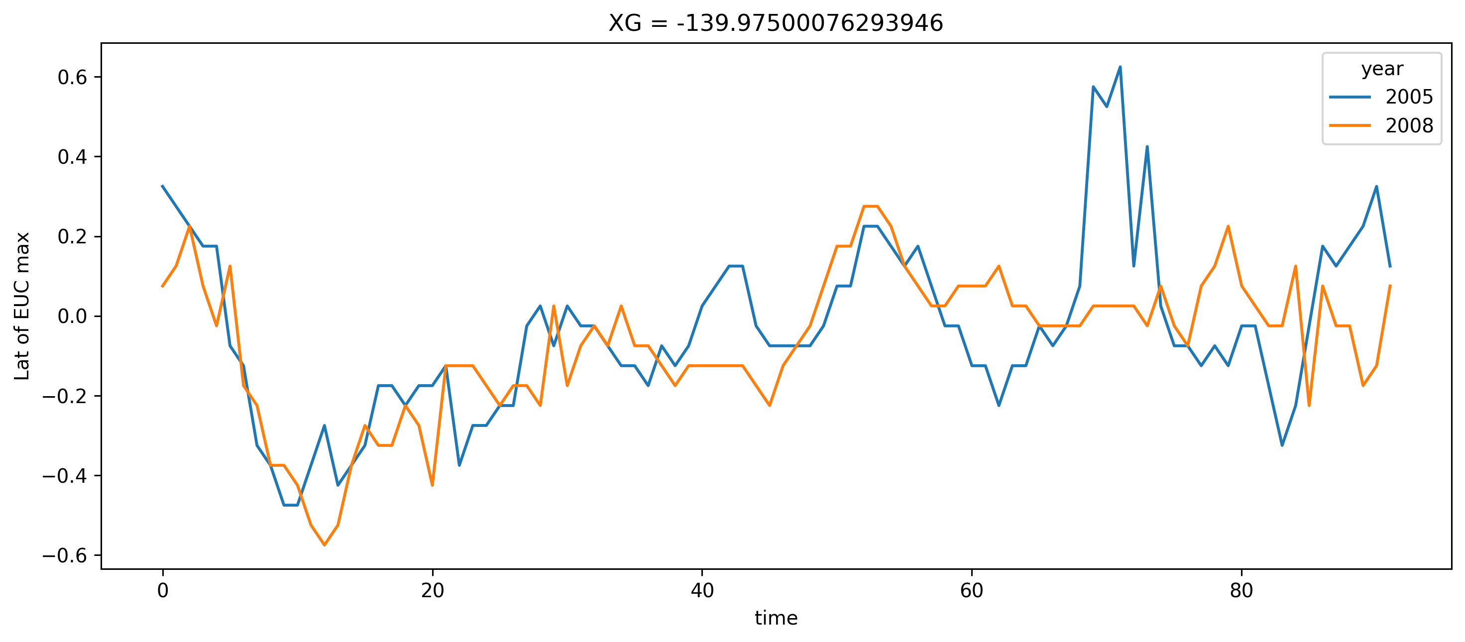
I think I want a metric for “TIW centroid” about the equator to judge if TIWs are further north during one season vs the other.
ds140 = dcpy.dask.map_copy(
ond0508[["theta", "u", "v", "w"]].cf.sel(X=-140, method="nearest")
).load()
fg = (
ds140.u.cf.sel(Z=slice(-250), YC=slice(-6, 6))
.mean("time")
.plot.contourf(col="year", robust=True, levels=np.arange(-1, 1.01, 0.05))
)
fg.map(lambda: plt.axvline(0, color="w"))
<xarray.plot.facetgrid.FacetGrid at 0x2af893d51640>
argmax = ds140.u.sel(YC=slice(-2.5, 2.5)).argmax(["YC", "RC"])
ds140.u.sel(YC=slice(-2.5, 2.5)).YC.isel(YC=argmax["YC"]).plot(
hue="year", size=5, aspect=2.5
)
plt.ylabel("Lat of EUC max")
Text(0, 0.5, 'Lat of EUC max')
f, ax = plt.subplots(1, 2, sharey=True)
ds140.theta.cf.sel(Z=slice(-50)).cf.mean("Z").mean("time").plot(
hue="year", y="YC", ax=ax[0]
)
(ds140.v**2 / 2).cf.sel(Z=slice(-50)).cf.mean(["Z", "time"]).plot(hue="year", y="YG")
ax[1].set_xlabel("$v^2/2$")
Text(0.5, 0, '$v^2/2$')
ds140.theta.cf.sel(Z=slice(-50)).cf.mean("Z").plot(
robust=True, row="year", aspect=2, x="time"
)
<xarray.plot.facetgrid.FacetGrid at 0x2af82cf3a580>
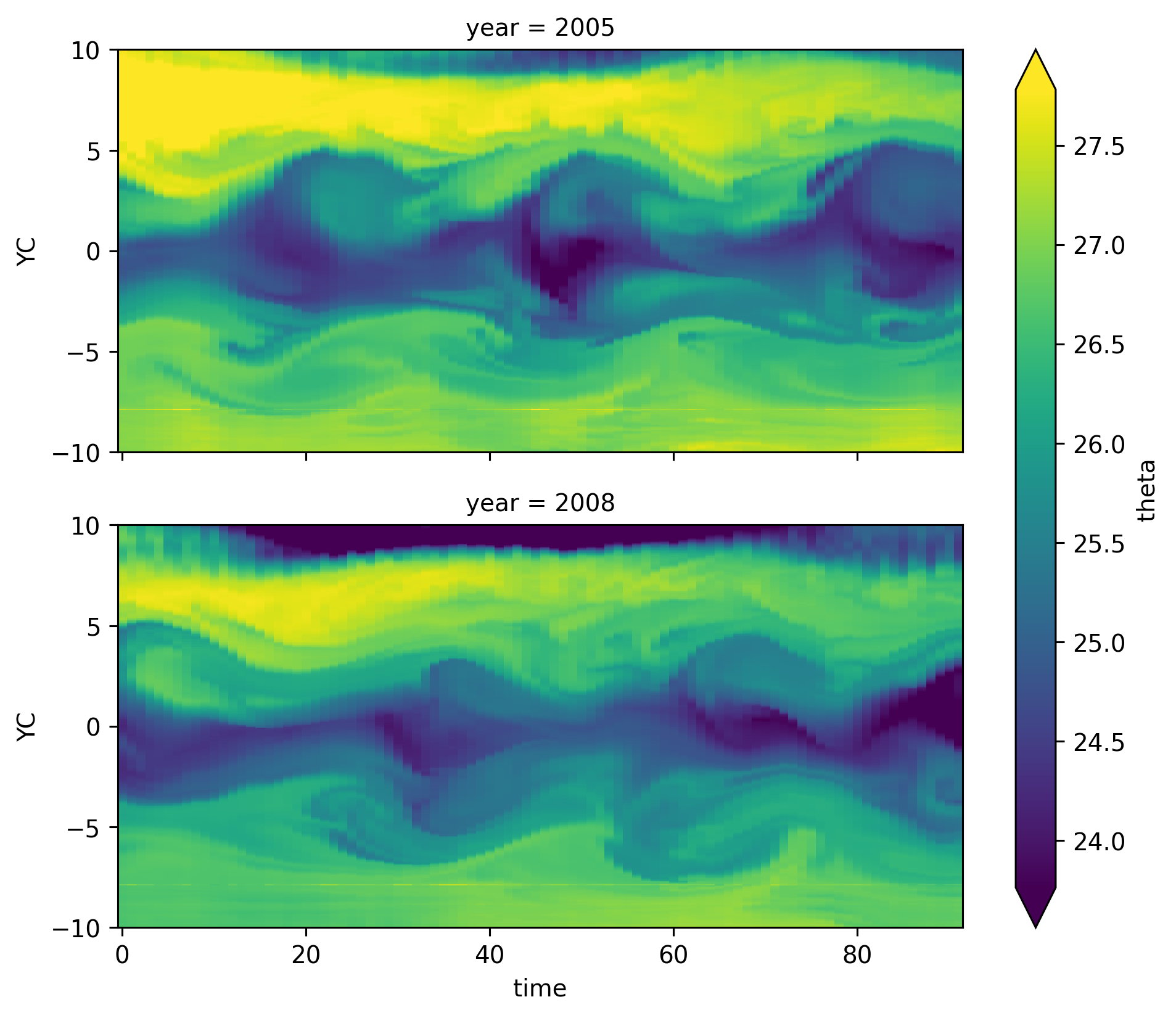
Cold tongue is in basically the same place
MLD#
meanmld = (
ond0508.mld.sel(XC=-140, method="nearest")
.sel(YC=slice(-0.5, 0.5))
.mean("YC")
.load()
)
meanmld.plot(hue="year", size=5, aspect=2.5)
plt.title("140°W, 0.5°S-0.5°N mean")
Text(0.5, 1.0, '140°W, 0.5°S-0.5°N mean')
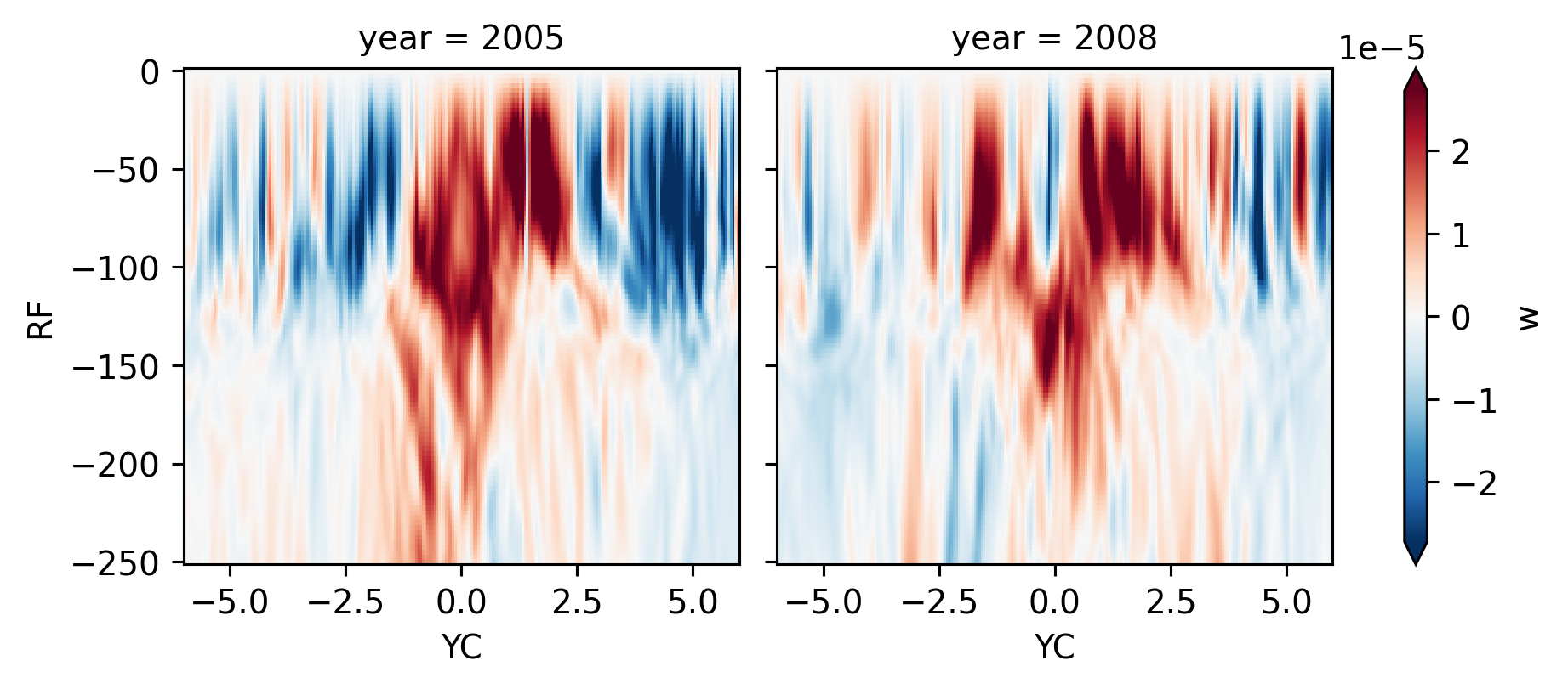
w#
Note near-equatorial downwelling in 2008
ds140.w.sel(RF=slice(-250), YC=slice(-6, 6)).mean("time").plot(col="year", robust=True)
<xarray.plot.facetgrid.FacetGrid at 0x2afdda761df0>
def plot_w(w):
slider = pnw.DiscreteSlider # pnw.IntSlider(start=0, end=92)
return (
w.sel(RF=-50, method="nearest")
.interactive.sel(time=slider)
.hvplot(clim=(-3e-4, 3e-4), cmap="RdBu_r")
)
wplot08 = plot_w(ond08.w)
wplot05 = plot_w(ond05.w)
wplot05 * (hv.HLine(0) * hv.VLine(-140))
wplot08 * (hv.HLine(0) * hv.VLine(-140))
w05 = ond05.w.sel(XC=[-155, -140, -125, -110], method="nearest").load()
w08 = ond08.w.sel(XC=[-155, -140, -125, -110], method="nearest").load()
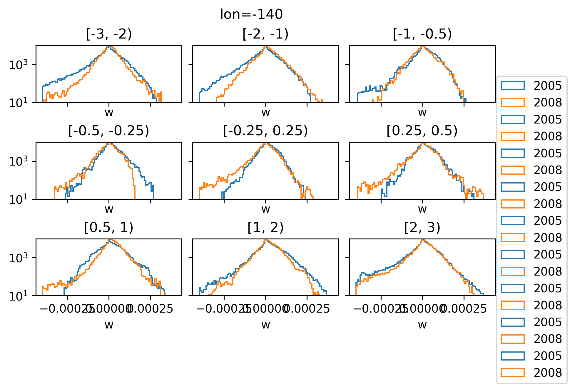
w histograms by latitude#
It looked like 2005 had more positive w; BUT once I change to log scale on the y-axis; it looks like 2008 has a lot more intense -ve w.
The more intense -ve w is in 0.5S - 0.5N
Are the TIWs in different places?
At first I thought regridding to a y_EUC centered coordinate would help but it looks like the EUC max is in roughly the same place.
I think I need a measure of TIW centroids or something?
Show code cell source
def plot_w_hist(*w, lon):
kwargs = dict(bins=np.linspace(-4e-4, 4e-4, 100), histtype="step", density=True)
breaks = [-3, -2, -1, -0.5, -0.25, 0.25, 0.5, 1, 2, 3]
f, axes = plt.subplots(3, 3, sharex=True, sharey=True, constrained_layout=True)
for ax, (left, right) in zip(axes.flat, zip(breaks[:-1], breaks[1:])):
sel = lambda x: x.cf.sel(X=lon, method="nearest").sel(
YC=slice(left, right), RF=slice(-100)
)
for w_ in w:
w_.pipe(sel).plot.hist(
**kwargs,
label=str(w_.time.dt.year.data[0]),
ax=ax,
yscale="log",
ylim=(1e1, 1e4),
)
ax.set_title(f"[{left!r}, {right!r})")
f.legend(bbox_to_anchor=(1.15, 0.8))
f.suptitle(f"lon={lon}")
dcpy.plots.clean_axes(ax)
plot_w_hist(w05, w08, lon=-140)
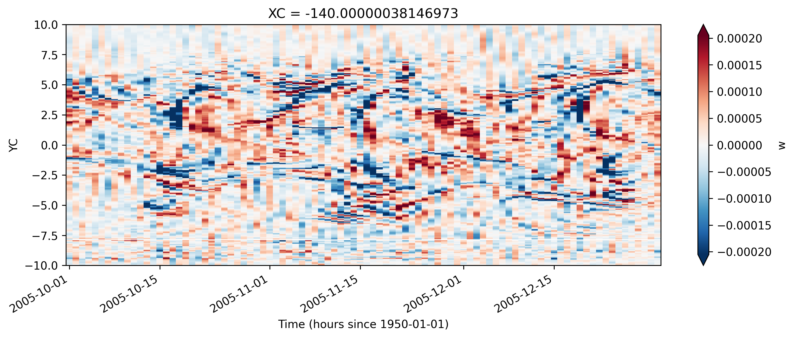
TIWs, divergence terms, w#
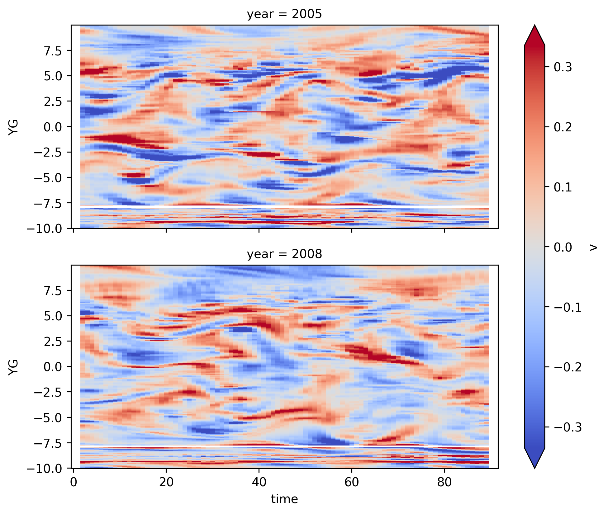
The w field is messy
Smoothed v and ∂v/∂y line up nicely
w05.cf.sel(Z=slice(-50, -100)).sel(XC=-140, method="nearest").cf.mean("Z").plot(
x="time", robust=True, size=4, aspect=3
)
w08.cf.sel(Z=slice(-50, -100)).sel(XC=-140, method="nearest").cf.mean("Z").plot(
x="time", robust=True, size=4, aspect=3
)
<matplotlib.collections.QuadMesh at 0x2afd9360b5e0>
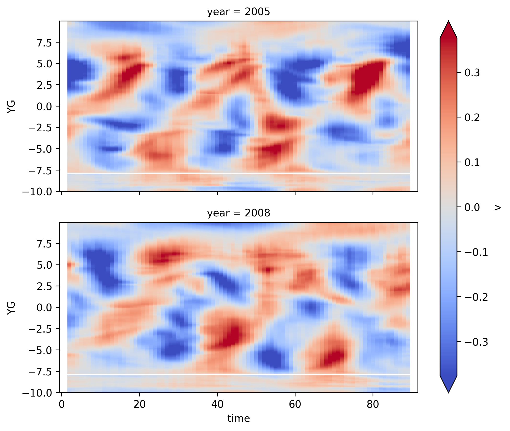
v#
shows nice phase signature and TIWs “leaning” into the SEC-EUC zonal flow
fg = (
ds140.v.cf.sel(Z=slice(-30, -100))
.cf.mean("Z")
.rolling(time=5, center=True)
.mean()
.plot(robust=True, row="year", aspect=2, x="time", cmap=mpl.cm.coolwarm)
)
∂v/∂y#
fg = (
ds140.v.cf.differentiate("Y")
.cf.sel(Z=slice(-30, -100))
.cf.mean("Z")
.rolling(time=5, center=True)
.mean()
.plot(robust=True, row="year", aspect=2, x="time", cmap=mpl.cm.coolwarm)
)
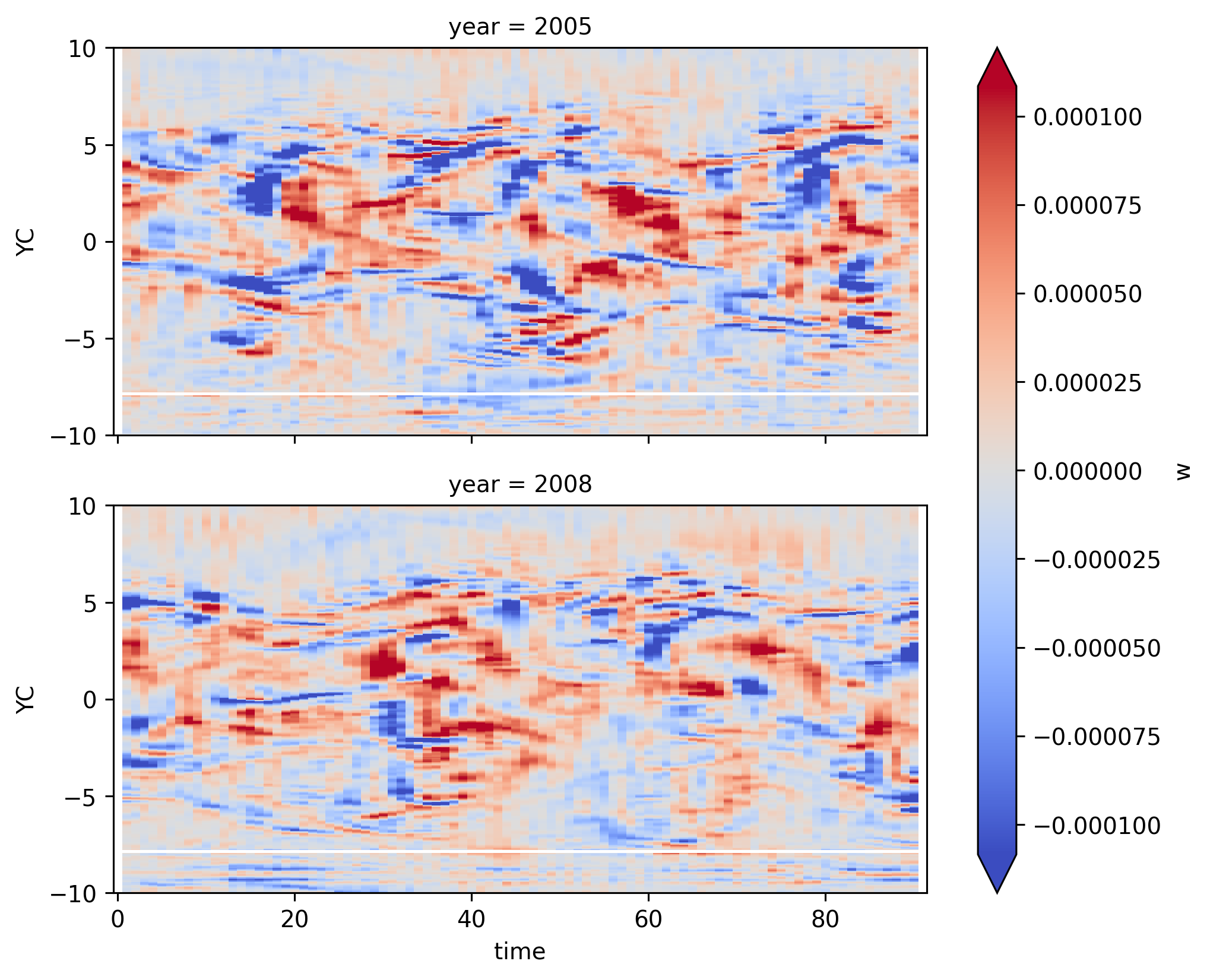
w#
smoothing the w field helps a bit; see downwelling followed by upwelling TIW pattern
fg = (
ds140.w.cf.sel(Z=slice(-40, -120))
.cf.mean("Z")
.rolling(time=3, YC=3, center=True)
.mean()
.plot(robust=True, row="year", aspect=2, x="time", cmap=mpl.cm.coolwarm)
)
fg.data = (
ds140.v.cf.differentiate("Y")
.cf.sel(Z=slice(-40, -100))
.cf.mean("Z")
.rolling(time=5, YG=5, center=True)
.mean()
)
# fg.map_dataarray(
# xr.plot.contour,
# x="time",
# y="YG",
# levels=5,
# cmap=mpl.cm.PuOr_r,
# linewidths=1,
# robust=True,
# add_colorbar=False,
# )
I started looking to see if there was a dominant contributor to \(u_x + v_y\) but not clear
ux = grid.derivative(ond05.isel(time=50).u, "X").load()
vy = grid.derivative(ond05.isel(time=50).v, "Y").load()
/glade/u/home/dcherian/python/xgcm/xgcm/grid.py:1384: UserWarning: Metric at ('RC', 'YC', 'XC') being interpolated from metrics at dimensions ('YG', 'XC'). Boundary value set to 'extend'.
warnings.warn(
/glade/u/home/dcherian/python/xgcm/xgcm/grid.py:1384: UserWarning: Metric at ('RC', 'YC', 'XC') being interpolated from metrics at dimensions ('YG', 'XC'). Boundary value set to 'extend'.
warnings.warn(
div = xr.concat([ux, vy], dim="div")
div["div"] = ["ux", "vy"]
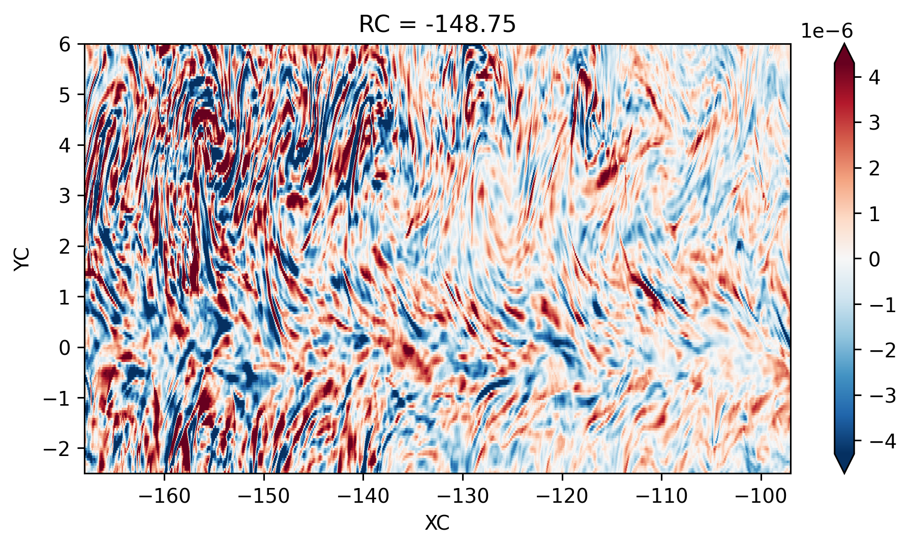
(ux + vy).sel(RC=-150, method="nearest").plot(
robust=True,
add_colorbar=True,
# vmin=-1,
# vmax=1,
cmap=mpl.cm.RdBu_r,
aspect=2,
size=4,
ylim=(-2.5, 6),
)
<matplotlib.collections.QuadMesh at 0x2afd91decd90>
Single TIW period: 2021 paper#
period4 = xr.open_zarr(
"/glade/work/dcherian/pump/zarrs/110w-period-4-3.zarr", consolidated=True
)
del period4["time"].attrs["long_name"]
central = period4.isel(longitude=1)
metrics = (
pump.model.read_metrics(
f"/glade/campaign/cgd/oce/people/dcherian/TPOS_MITgcm_1_hb/"
)
.reindex_like(central.expand_dims("longitude"), method="nearest")
.load()
).squeeze()
/glade/u/home/dcherian/miniconda3/envs/dcpy/lib/python3.8/site-packages/xarray/core/indexing.py:1375: PerformanceWarning: Slicing is producing a large chunk. To accept the large
chunk and silence this warning, set the option
>>> with dask.config.set(**{'array.slicing.split_large_chunks': False}):
... array[indexer]
To avoid creating the large chunks, set the option
>>> with dask.config.set(**{'array.slicing.split_large_chunks': True}):
... array[indexer]
value = value[(slice(None),) * axis + (subkey,)]
central["Jq"] = (
1035 * 3994 * (central.DFrI_TH + central.KPPg_TH.fillna(0)) / metrics.RAC
)
central["time"] = central["time"] - pd.Timedelta("7h")
central["dens"] = pump.mdjwf.dens(central.salt, central.theta, np.array([0.0]))
central = pump.calc.calc_reduced_shear(central)
central["mld"] = pump.calc.get_mld(central.dens)
central["dcl_base"] = pump.calc.get_dcl_base_Ri(central)
central["dcl"] = central["mld"] - central["dcl_base"]
central["sst"] = central.theta.isel(depth=0)
central["eucmax"] = pump.calc.get_euc_max(
central.u.sel(latitude=0, method="nearest", drop=True)
)
central.depth.attrs["units"] = "m"
central.Jq.attrs["long_name"] = "$J^t_q$"
central.Jq.attrs["units"] = "W/m²"
central.S2.attrs["long_name"] = "$S²$"
central.S2.attrs["units"] = "$s^{-2}$"
central.Ri.attrs["long_name"] = "$Ri$"
central.N2.attrs["long_name"] = "$N²$"
central.N2.attrs["units"] = "$s^{-2}$"
central
calc uz
calc vz
calc S2
calc N2
calc shred2
Calc Ri
<xarray.Dataset>
Dimensions: (depth: 200, latitude: 400, time: 779)
Coordinates:
* depth (depth) float32 -0.5 -1.5 -2.5 -3.5 ... -197.5 -198.5 -199.5
* latitude (latitude) float32 -10.0 -9.95 -9.9 -9.85 ... 9.85 9.9 9.95 10.0
longitude float32 -110.0
* time (time) datetime64[ns] 1995-11-14T17:00:00 ... 1995-12-17T03:00:00
Data variables:
DFrI_TH (time, depth, latitude) float32 dask.array<chunksize=(1, 200, 400), meta=np.ndarray>
ETAN (time, latitude) float32 dask.array<chunksize=(1, 400), meta=np.ndarray>
KPPRi (time, depth, latitude) float32 dask.array<chunksize=(1, 200, 400), meta=np.ndarray>
KPPbo (time, latitude) float32 dask.array<chunksize=(1, 400), meta=np.ndarray>
KPPdiffT (time, depth, latitude) float32 dask.array<chunksize=(1, 200, 400), meta=np.ndarray>
KPPg_TH (time, depth, latitude) float32 dask.array<chunksize=(1, 200, 400), meta=np.ndarray>
KPPhbl (time, latitude) float32 dask.array<chunksize=(1, 400), meta=np.ndarray>
KPPviscA (time, depth, latitude) float32 dask.array<chunksize=(1, 200, 400), meta=np.ndarray>
Um_Diss (time, depth, latitude) float32 dask.array<chunksize=(1, 200, 400), meta=np.ndarray>
VISrI_Um (time, depth, latitude) float32 dask.array<chunksize=(1, 200, 400), meta=np.ndarray>
VISrI_Vm (time, depth, latitude) float32 dask.array<chunksize=(1, 200, 400), meta=np.ndarray>
Vm_Diss (time, depth, latitude) float32 dask.array<chunksize=(1, 200, 400), meta=np.ndarray>
salt (time, depth, latitude) float32 dask.array<chunksize=(1, 200, 400), meta=np.ndarray>
theta (time, depth, latitude) float32 dask.array<chunksize=(1, 200, 400), meta=np.ndarray>
u (time, depth, latitude) float32 dask.array<chunksize=(1, 200, 400), meta=np.ndarray>
v (time, depth, latitude) float32 dask.array<chunksize=(1, 200, 400), meta=np.ndarray>
w (time, depth, latitude) float32 dask.array<chunksize=(1, 200, 400), meta=np.ndarray>
Jq (time, depth, latitude) float64 dask.array<chunksize=(1, 200, 400), meta=np.ndarray>
dens (time, depth, latitude) float64 dask.array<chunksize=(1, 200, 400), meta=np.ndarray>
uz (time, depth, latitude) float32 dask.array<chunksize=(1, 200, 400), meta=np.ndarray>
vz (time, depth, latitude) float32 dask.array<chunksize=(1, 200, 400), meta=np.ndarray>
S2 (time, depth, latitude) float32 dask.array<chunksize=(1, 200, 400), meta=np.ndarray>
shear (time, depth, latitude) float32 dask.array<chunksize=(1, 200, 400), meta=np.ndarray>
N2 (time, depth, latitude) float64 dask.array<chunksize=(1, 200, 400), meta=np.ndarray>
shred2 (time, depth, latitude) float64 dask.array<chunksize=(1, 200, 400), meta=np.ndarray>
Ri (time, depth, latitude) float64 dask.array<chunksize=(1, 200, 400), meta=np.ndarray>
mld (time, latitude) float32 dask.array<chunksize=(1, 400), meta=np.ndarray>
dcl_base (time, latitude) float32 dask.array<chunksize=(1, 400), meta=np.ndarray>
dcl (time, latitude) float32 dask.array<chunksize=(1, 400), meta=np.ndarray>
sst (time, latitude) float32 dask.array<chunksize=(1, 400), meta=np.ndarray>
eucmax (time) float32 -97.5 -97.5 -97.5 -97.5 ... -100.5 -99.5 -99.5
Attributes:
easting: longitude
field_julian_date: 400296
julian_day_unit: days since 1950-01-01 00:00:00
northing: latitude
title: daily snapshot from 1/20 degree Equatorial Pacific MI...- depth: 200
- latitude: 400
- time: 779
- depth(depth)float32-0.5 -1.5 -2.5 ... -198.5 -199.5
- units :
- m
array([ -0.5, -1.5, -2.5, -3.5, -4.5, -5.5, -6.5, -7.5, -8.5, -9.5, -10.5, -11.5, -12.5, -13.5, -14.5, -15.5, -16.5, -17.5, -18.5, -19.5, -20.5, -21.5, -22.5, -23.5, -24.5, -25.5, -26.5, -27.5, -28.5, -29.5, -30.5, -31.5, -32.5, -33.5, -34.5, -35.5, -36.5, -37.5, -38.5, -39.5, -40.5, -41.5, -42.5, -43.5, -44.5, -45.5, -46.5, -47.5, -48.5, -49.5, -50.5, -51.5, -52.5, -53.5, -54.5, -55.5, -56.5, -57.5, -58.5, -59.5, -60.5, -61.5, -62.5, -63.5, -64.5, -65.5, -66.5, -67.5, -68.5, -69.5, -70.5, -71.5, -72.5, -73.5, -74.5, -75.5, -76.5, -77.5, -78.5, -79.5, -80.5, -81.5, -82.5, -83.5, -84.5, -85.5, -86.5, -87.5, -88.5, -89.5, -90.5, -91.5, -92.5, -93.5, -94.5, -95.5, -96.5, -97.5, -98.5, -99.5, -100.5, -101.5, -102.5, -103.5, -104.5, -105.5, -106.5, -107.5, -108.5, -109.5, -110.5, -111.5, -112.5, -113.5, -114.5, -115.5, -116.5, -117.5, -118.5, -119.5, -120.5, -121.5, -122.5, -123.5, -124.5, -125.5, -126.5, -127.5, -128.5, -129.5, -130.5, -131.5, -132.5, -133.5, -134.5, -135.5, -136.5, -137.5, -138.5, -139.5, -140.5, -141.5, -142.5, -143.5, -144.5, -145.5, -146.5, -147.5, -148.5, -149.5, -150.5, -151.5, -152.5, -153.5, -154.5, -155.5, -156.5, -157.5, -158.5, -159.5, -160.5, -161.5, -162.5, -163.5, -164.5, -165.5, -166.5, -167.5, -168.5, -169.5, -170.5, -171.5, -172.5, -173.5, -174.5, -175.5, -176.5, -177.5, -178.5, -179.5, -180.5, -181.5, -182.5, -183.5, -184.5, -185.5, -186.5, -187.5, -188.5, -189.5, -190.5, -191.5, -192.5, -193.5, -194.5, -195.5, -196.5, -197.5, -198.5, -199.5], dtype=float32) - latitude(latitude)float32-10.0 -9.95 -9.9 ... 9.9 9.95 10.0
array([-10. , -9.949875, -9.89975 , ..., 9.89975 , 9.949875, 10. ], dtype=float32) - longitude()float32-110.0
array(-110.00916, dtype=float32)
- time(time)datetime64[ns]1995-11-14T17:00:00 ... 1995-12-...
- _CoordinateAxisType :
- Time
- axis :
- T
- standard_name :
- time
array(['1995-11-14T17:00:00.000000000', '1995-11-14T18:00:00.000000000', '1995-11-14T19:00:00.000000000', ..., '1995-12-17T01:00:00.000000000', '1995-12-17T02:00:00.000000000', '1995-12-17T03:00:00.000000000'], dtype='datetime64[ns]')
- DFrI_TH(time, depth, latitude)float32dask.array<chunksize=(1, 200, 400), meta=np.ndarray>
Array Chunk Bytes 249.28 MB 320.00 kB Shape (779, 200, 400) (1, 200, 400) Count 1559 Tasks 779 Chunks Type float32 numpy.ndarray - ETAN(time, latitude)float32dask.array<chunksize=(1, 400), meta=np.ndarray>
Array Chunk Bytes 1.25 MB 1.60 kB Shape (779, 400) (1, 400) Count 1559 Tasks 779 Chunks Type float32 numpy.ndarray - KPPRi(time, depth, latitude)float32dask.array<chunksize=(1, 200, 400), meta=np.ndarray>
Array Chunk Bytes 249.28 MB 320.00 kB Shape (779, 200, 400) (1, 200, 400) Count 1559 Tasks 779 Chunks Type float32 numpy.ndarray - KPPbo(time, latitude)float32dask.array<chunksize=(1, 400), meta=np.ndarray>
Array Chunk Bytes 1.25 MB 1.60 kB Shape (779, 400) (1, 400) Count 1559 Tasks 779 Chunks Type float32 numpy.ndarray - KPPdiffT(time, depth, latitude)float32dask.array<chunksize=(1, 200, 400), meta=np.ndarray>
Array Chunk Bytes 249.28 MB 320.00 kB Shape (779, 200, 400) (1, 200, 400) Count 1559 Tasks 779 Chunks Type float32 numpy.ndarray - KPPg_TH(time, depth, latitude)float32dask.array<chunksize=(1, 200, 400), meta=np.ndarray>
Array Chunk Bytes 249.28 MB 320.00 kB Shape (779, 200, 400) (1, 200, 400) Count 1559 Tasks 779 Chunks Type float32 numpy.ndarray - KPPhbl(time, latitude)float32dask.array<chunksize=(1, 400), meta=np.ndarray>
Array Chunk Bytes 1.25 MB 1.60 kB Shape (779, 400) (1, 400) Count 1559 Tasks 779 Chunks Type float32 numpy.ndarray - KPPviscA(time, depth, latitude)float32dask.array<chunksize=(1, 200, 400), meta=np.ndarray>
Array Chunk Bytes 249.28 MB 320.00 kB Shape (779, 200, 400) (1, 200, 400) Count 1559 Tasks 779 Chunks Type float32 numpy.ndarray - Um_Diss(time, depth, latitude)float32dask.array<chunksize=(1, 200, 400), meta=np.ndarray>
Array Chunk Bytes 249.28 MB 320.00 kB Shape (779, 200, 400) (1, 200, 400) Count 1559 Tasks 779 Chunks Type float32 numpy.ndarray - VISrI_Um(time, depth, latitude)float32dask.array<chunksize=(1, 200, 400), meta=np.ndarray>
Array Chunk Bytes 249.28 MB 320.00 kB Shape (779, 200, 400) (1, 200, 400) Count 1559 Tasks 779 Chunks Type float32 numpy.ndarray - VISrI_Vm(time, depth, latitude)float32dask.array<chunksize=(1, 200, 400), meta=np.ndarray>
Array Chunk Bytes 249.28 MB 320.00 kB Shape (779, 200, 400) (1, 200, 400) Count 1559 Tasks 779 Chunks Type float32 numpy.ndarray - Vm_Diss(time, depth, latitude)float32dask.array<chunksize=(1, 200, 400), meta=np.ndarray>
Array Chunk Bytes 249.28 MB 320.00 kB Shape (779, 200, 400) (1, 200, 400) Count 1559 Tasks 779 Chunks Type float32 numpy.ndarray - salt(time, depth, latitude)float32dask.array<chunksize=(1, 200, 400), meta=np.ndarray>
Array Chunk Bytes 249.28 MB 320.00 kB Shape (779, 200, 400) (1, 200, 400) Count 1559 Tasks 779 Chunks Type float32 numpy.ndarray - theta(time, depth, latitude)float32dask.array<chunksize=(1, 200, 400), meta=np.ndarray>
Array Chunk Bytes 249.28 MB 320.00 kB Shape (779, 200, 400) (1, 200, 400) Count 1559 Tasks 779 Chunks Type float32 numpy.ndarray - u(time, depth, latitude)float32dask.array<chunksize=(1, 200, 400), meta=np.ndarray>
Array Chunk Bytes 249.28 MB 320.00 kB Shape (779, 200, 400) (1, 200, 400) Count 1559 Tasks 779 Chunks Type float32 numpy.ndarray - v(time, depth, latitude)float32dask.array<chunksize=(1, 200, 400), meta=np.ndarray>
Array Chunk Bytes 249.28 MB 320.00 kB Shape (779, 200, 400) (1, 200, 400) Count 1559 Tasks 779 Chunks Type float32 numpy.ndarray - w(time, depth, latitude)float32dask.array<chunksize=(1, 200, 400), meta=np.ndarray>
Array Chunk Bytes 249.28 MB 320.00 kB Shape (779, 200, 400) (1, 200, 400) Count 1559 Tasks 779 Chunks Type float32 numpy.ndarray - Jq(time, depth, latitude)float64dask.array<chunksize=(1, 200, 400), meta=np.ndarray>
- long_name :
- $J^t_q$
- units :
- W/m²
Array Chunk Bytes 498.56 MB 640.00 kB Shape (779, 200, 400) (1, 200, 400) Count 7793 Tasks 779 Chunks Type float64 numpy.ndarray - dens(time, depth, latitude)float64dask.array<chunksize=(1, 200, 400), meta=np.ndarray>
Array Chunk Bytes 498.56 MB 640.00 kB Shape (779, 200, 400) (1, 200, 400) Count 5456 Tasks 779 Chunks Type float64 numpy.ndarray - uz(time, depth, latitude)float32dask.array<chunksize=(1, 200, 400), meta=np.ndarray>
Array Chunk Bytes 249.28 MB 320.00 kB Shape (779, 200, 400) (1, 200, 400) Count 6233 Tasks 779 Chunks Type float32 numpy.ndarray - vz(time, depth, latitude)float32dask.array<chunksize=(1, 200, 400), meta=np.ndarray>
Array Chunk Bytes 249.28 MB 320.00 kB Shape (779, 200, 400) (1, 200, 400) Count 6233 Tasks 779 Chunks Type float32 numpy.ndarray - S2(time, depth, latitude)float32dask.array<chunksize=(1, 200, 400), meta=np.ndarray>
- long_name :
- $S²$
- units :
- $s^{-2}$
Array Chunk Bytes 249.28 MB 320.00 kB Shape (779, 200, 400) (1, 200, 400) Count 14803 Tasks 779 Chunks Type float32 numpy.ndarray - shear(time, depth, latitude)float32dask.array<chunksize=(1, 200, 400), meta=np.ndarray>
- long_name :
- |$u_z$|
- units :
- s$^{-1}$
Array Chunk Bytes 249.28 MB 320.00 kB Shape (779, 200, 400) (1, 200, 400) Count 15582 Tasks 779 Chunks Type float32 numpy.ndarray - N2(time, depth, latitude)float64dask.array<chunksize=(1, 200, 400), meta=np.ndarray>
- long_name :
- $N²$
- units :
- $s^{-2}$
Array Chunk Bytes 498.56 MB 640.00 kB Shape (779, 200, 400) (1, 200, 400) Count 10909 Tasks 779 Chunks Type float64 numpy.ndarray - shred2(time, depth, latitude)float64dask.array<chunksize=(1, 200, 400), meta=np.ndarray>
- long_name :
- Reduced shear$^2$
- units :
- $s^{-2}$
Array Chunk Bytes 498.56 MB 640.00 kB Shape (779, 200, 400) (1, 200, 400) Count 27270 Tasks 779 Chunks Type float64 numpy.ndarray - Ri(time, depth, latitude)float64dask.array<chunksize=(1, 200, 400), meta=np.ndarray>
- long_name :
- $Ri$
- units :
Array Chunk Bytes 498.56 MB 640.00 kB Shape (779, 200, 400) (1, 200, 400) Count 26491 Tasks 779 Chunks Type float64 numpy.ndarray - mld(time, latitude)float32dask.array<chunksize=(1, 400), meta=np.ndarray>
- long_name :
- MLD
- units :
- m
- description :
- Interpolate density to 1m grid. Search for max depth where |drho| > 0.01 and N2 > 1e-5
Array Chunk Bytes 1.25 MB 1.60 kB Shape (779, 400) (1, 400) Count 19479 Tasks 779 Chunks Type float32 numpy.ndarray - dcl_base(time, latitude)float32dask.array<chunksize=(1, 400), meta=np.ndarray>
- long_name :
- DCL Base (Ri)
- units :
- m
- description :
- Deepest depth above EUC where Ri=0.54
Array Chunk Bytes 1.25 MB 1.60 kB Shape (779, 400) (1, 400) Count 67018 Tasks 779 Chunks Type float32 numpy.ndarray - dcl(time, latitude)float32dask.array<chunksize=(1, 400), meta=np.ndarray>
- long_name :
- MLD
- units :
- m
- description :
- Interpolate density to 1m grid. Search for max depth where |drho| > 0.01 and N2 > 1e-5
Array Chunk Bytes 1.25 MB 1.60 kB Shape (779, 400) (1, 400) Count 67797 Tasks 779 Chunks Type float32 numpy.ndarray - sst(time, latitude)float32dask.array<chunksize=(1, 400), meta=np.ndarray>
Array Chunk Bytes 1.25 MB 1.60 kB Shape (779, 400) (1, 400) Count 2338 Tasks 779 Chunks Type float32 numpy.ndarray - eucmax(time)float32-97.5 -97.5 -97.5 ... -99.5 -99.5
- long_name :
- Depth of EUC max
- units :
- m
array([ -97.5, -97.5, -97.5, -97.5, -97.5, -97.5, -96.5, -96.5, -96.5, -96.5, -95.5, -95.5, -95.5, -95.5, -94.5, -94.5, -94.5, -94.5, -93.5, -93.5, -93.5, -93.5, -92.5, -92.5, -91.5, -91.5, -91.5, -90.5, -90.5, -89.5, -89.5, -89.5, -89.5, -88.5, -88.5, -88.5, -88.5, -88.5, -88.5, -88.5, -88.5, -88.5, -88.5, -89.5, -89.5, -89.5, -89.5, -90.5, -90.5, -90.5, -90.5, -90.5, -90.5, -90.5, -90.5, -90.5, -90.5, -90.5, -89.5, -89.5, -88.5, -88.5, -87.5, -87.5, -87.5, -86.5, -86.5, -85.5, -85.5, -85.5, -85.5, -85.5, -85.5, -85.5, -85.5, -85.5, -85.5, -86.5, -86.5, -86.5, -86.5, -86.5, -86.5, -87.5, -87.5, -87.5, -87.5, -88.5, -88.5, -88.5, -88.5, -89.5, -89.5, -89.5, -89.5, -89.5, -89.5, -89.5, -89.5, -89.5, -89.5, -89.5, -89.5, -89.5, -89.5, -89.5, -90.5, -90.5, -90.5, -90.5, -90.5, -90.5, -90.5, -90.5, -90.5, -90.5, -90.5, -90.5, -89.5, -86.5, -85.5, -84.5, -83.5, -83.5, -82.5, -81.5, -80.5, -80.5, -79.5, -78.5, -78.5, -77.5, -77.5, -77.5, -76.5, -76.5, -76.5, -76.5, -76.5, -77.5, -77.5, -77.5, -78.5, -78.5, -78.5, -78.5, -78.5, -78.5, -78.5, -78.5, -78.5, -78.5, -78.5, -78.5, -78.5, -78.5, -78.5, -78.5, -78.5, -90.5, ... -80.5, -80.5, -79.5, -79.5, -79.5, -78.5, -78.5, -78.5, -77.5, -77.5, -77.5, -76.5, -76.5, -76.5, -76.5, -75.5, -75.5, -75.5, -75.5, -75.5, -75.5, -75.5, -75.5, -75.5, -75.5, -75.5, -75.5, -75.5, -75.5, -76.5, -76.5, -76.5, -76.5, -76.5, -76.5, -76.5, -76.5, -76.5, -76.5, -76.5, -76.5, -76.5, -76.5, -76.5, -76.5, -77.5, -77.5, -77.5, -77.5, -78.5, -78.5, -78.5, -78.5, -79.5, -79.5, -79.5, -79.5, -79.5, -80.5, -80.5, -80.5, -80.5, -80.5, -81.5, -81.5, -81.5, -81.5, -81.5, -82.5, -82.5, -82.5, -83.5, -83.5, -83.5, -84.5, -84.5, -85.5, -85.5, -85.5, -86.5, -86.5, -86.5, -87.5, -87.5, -88.5, -88.5, -89.5, -89.5, -90.5, -90.5, -91.5, -91.5, -91.5, -91.5, -91.5, -91.5, -92.5, -92.5, -92.5, -92.5, -93.5, -93.5, -93.5, -93.5, -93.5, -94.5, -94.5, -94.5, -94.5, -94.5, -94.5, -94.5, -94.5, -94.5, -95.5, -95.5, -95.5, -95.5, -95.5, -95.5, -95.5, -95.5, -95.5, -95.5, -94.5, -94.5, -94.5, -94.5, -94.5, -94.5, -94.5, -93.5, -93.5, -93.5, -93.5, -93.5, -92.5, -92.5, -92.5, -92.5, -92.5, -92.5, -92.5, -91.5, -91.5, -91.5, -102.5, -102.5, -102.5, -101.5, -101.5, -100.5, -100.5, -99.5, -99.5], dtype=float32)
- easting :
- longitude
- field_julian_date :
- 400296
- julian_day_unit :
- days since 1950-01-01 00:00:00
- northing :
- latitude
- title :
- daily snapshot from 1/20 degree Equatorial Pacific MITgcm simulation
central.w.load()
<xarray.DataArray 'w' (time: 779, depth: 200, latitude: 400, longitude: 3)>
array([[[[-8.32392686e-07, -8.61631122e-07, -9.07944013e-07],
[-8.17283251e-07, -8.39938480e-07, -8.78521575e-07],
[-8.14519808e-07, -8.35834385e-07, -8.55945700e-07],
...,
[-2.07602127e-07, -2.00864179e-07, -1.98754080e-07],
[-2.06921740e-07, -2.26620955e-07, -2.43814696e-07],
[-1.80513695e-07, -2.17974403e-07, -2.52572022e-07]],
[[-2.42294459e-06, -3.05959338e-06, -3.24233270e-06],
[-2.51864435e-06, -3.08625977e-06, -3.58562716e-06],
[-2.49380400e-06, -3.41150280e-06, -3.97996473e-06],
...,
[ 2.10747203e-06, 1.65012580e-06, 1.15887929e-06],
[ 1.27279213e-06, 7.15527619e-07, 2.72692631e-07],
[-5.73148554e-07, -1.04561616e-06, -1.42848603e-06]],
[[-4.02487240e-06, -5.26639315e-06, -5.58513466e-06],
[-4.23122447e-06, -5.34199489e-06, -6.30122440e-06],
[-4.18542413e-06, -5.99460918e-06, -7.11171651e-06],
...,
...
[ 4.57714168e-06, 3.17592526e-06, -1.33422600e-05],
[-1.43890775e-05, -3.12485827e-05, -5.46250267e-05],
[-5.27998491e-05, -7.76431771e-05, -1.01270351e-04]],
[[ 3.85325366e-05, 2.63559486e-05, 1.21922913e-05],
[ 2.41746147e-05, 1.80613529e-06, -2.40914906e-05],
[ 5.65520440e-06, -2.40457211e-05, -4.94654341e-05],
...,
[ 4.26078304e-06, 2.97869406e-06, -1.33218573e-05],
[-1.47053061e-05, -3.17766717e-05, -5.48467360e-05],
[-5.34974752e-05, -7.84654549e-05, -1.01884856e-04]],
[[ 4.04056191e-05, 2.77295694e-05, 1.29975933e-05],
[ 2.59654771e-05, 3.19075821e-06, -2.32989441e-05],
[ 6.97214091e-06, -2.29840607e-05, -4.85406090e-05],
...,
[ 3.94934204e-06, 2.77228696e-06, -1.33081094e-05],
[-1.50320866e-05, -3.23151435e-05, -5.50692130e-05],
[-5.41884583e-05, -7.92831343e-05, -1.02494916e-04]]]],
dtype=float32)
Coordinates:
* depth (depth) float32 -0.5 -1.5 -2.5 -3.5 ... -197.5 -198.5 -199.5
* latitude (latitude) float32 -10.0 -9.95 -9.9 -9.85 ... 9.85 9.9 9.95 10.0
* longitude (longitude) float32 -110.1 -110.0 -110.0
* time (time) datetime64[ns] 1995-11-15 ... 1995-12-17T10:00:00- time: 779
- depth: 200
- latitude: 400
- longitude: 3
- -8.324e-07 -8.616e-07 -9.079e-07 ... -5.419e-05 -7.928e-05 -0.0001025
array([[[[-8.32392686e-07, -8.61631122e-07, -9.07944013e-07], [-8.17283251e-07, -8.39938480e-07, -8.78521575e-07], [-8.14519808e-07, -8.35834385e-07, -8.55945700e-07], ..., [-2.07602127e-07, -2.00864179e-07, -1.98754080e-07], [-2.06921740e-07, -2.26620955e-07, -2.43814696e-07], [-1.80513695e-07, -2.17974403e-07, -2.52572022e-07]], [[-2.42294459e-06, -3.05959338e-06, -3.24233270e-06], [-2.51864435e-06, -3.08625977e-06, -3.58562716e-06], [-2.49380400e-06, -3.41150280e-06, -3.97996473e-06], ..., [ 2.10747203e-06, 1.65012580e-06, 1.15887929e-06], [ 1.27279213e-06, 7.15527619e-07, 2.72692631e-07], [-5.73148554e-07, -1.04561616e-06, -1.42848603e-06]], [[-4.02487240e-06, -5.26639315e-06, -5.58513466e-06], [-4.23122447e-06, -5.34199489e-06, -6.30122440e-06], [-4.18542413e-06, -5.99460918e-06, -7.11171651e-06], ..., ... [ 4.57714168e-06, 3.17592526e-06, -1.33422600e-05], [-1.43890775e-05, -3.12485827e-05, -5.46250267e-05], [-5.27998491e-05, -7.76431771e-05, -1.01270351e-04]], [[ 3.85325366e-05, 2.63559486e-05, 1.21922913e-05], [ 2.41746147e-05, 1.80613529e-06, -2.40914906e-05], [ 5.65520440e-06, -2.40457211e-05, -4.94654341e-05], ..., [ 4.26078304e-06, 2.97869406e-06, -1.33218573e-05], [-1.47053061e-05, -3.17766717e-05, -5.48467360e-05], [-5.34974752e-05, -7.84654549e-05, -1.01884856e-04]], [[ 4.04056191e-05, 2.77295694e-05, 1.29975933e-05], [ 2.59654771e-05, 3.19075821e-06, -2.32989441e-05], [ 6.97214091e-06, -2.29840607e-05, -4.85406090e-05], ..., [ 3.94934204e-06, 2.77228696e-06, -1.33081094e-05], [-1.50320866e-05, -3.23151435e-05, -5.50692130e-05], [-5.41884583e-05, -7.92831343e-05, -1.02494916e-04]]]], dtype=float32) - depth(depth)float32-0.5 -1.5 -2.5 ... -198.5 -199.5
array([ -0.5, -1.5, -2.5, -3.5, -4.5, -5.5, -6.5, -7.5, -8.5, -9.5, -10.5, -11.5, -12.5, -13.5, -14.5, -15.5, -16.5, -17.5, -18.5, -19.5, -20.5, -21.5, -22.5, -23.5, -24.5, -25.5, -26.5, -27.5, -28.5, -29.5, -30.5, -31.5, -32.5, -33.5, -34.5, -35.5, -36.5, -37.5, -38.5, -39.5, -40.5, -41.5, -42.5, -43.5, -44.5, -45.5, -46.5, -47.5, -48.5, -49.5, -50.5, -51.5, -52.5, -53.5, -54.5, -55.5, -56.5, -57.5, -58.5, -59.5, -60.5, -61.5, -62.5, -63.5, -64.5, -65.5, -66.5, -67.5, -68.5, -69.5, -70.5, -71.5, -72.5, -73.5, -74.5, -75.5, -76.5, -77.5, -78.5, -79.5, -80.5, -81.5, -82.5, -83.5, -84.5, -85.5, -86.5, -87.5, -88.5, -89.5, -90.5, -91.5, -92.5, -93.5, -94.5, -95.5, -96.5, -97.5, -98.5, -99.5, -100.5, -101.5, -102.5, -103.5, -104.5, -105.5, -106.5, -107.5, -108.5, -109.5, -110.5, -111.5, -112.5, -113.5, -114.5, -115.5, -116.5, -117.5, -118.5, -119.5, -120.5, -121.5, -122.5, -123.5, -124.5, -125.5, -126.5, -127.5, -128.5, -129.5, -130.5, -131.5, -132.5, -133.5, -134.5, -135.5, -136.5, -137.5, -138.5, -139.5, -140.5, -141.5, -142.5, -143.5, -144.5, -145.5, -146.5, -147.5, -148.5, -149.5, -150.5, -151.5, -152.5, -153.5, -154.5, -155.5, -156.5, -157.5, -158.5, -159.5, -160.5, -161.5, -162.5, -163.5, -164.5, -165.5, -166.5, -167.5, -168.5, -169.5, -170.5, -171.5, -172.5, -173.5, -174.5, -175.5, -176.5, -177.5, -178.5, -179.5, -180.5, -181.5, -182.5, -183.5, -184.5, -185.5, -186.5, -187.5, -188.5, -189.5, -190.5, -191.5, -192.5, -193.5, -194.5, -195.5, -196.5, -197.5, -198.5, -199.5], dtype=float32) - latitude(latitude)float32-10.0 -9.95 -9.9 ... 9.9 9.95 10.0
array([-10. , -9.949875, -9.89975 , ..., 9.89975 , 9.949875, 10. ], dtype=float32) - longitude(longitude)float32-110.1 -110.0 -110.0
array([-110.0592 , -110.00916, -109.95913], dtype=float32)
- time(time)datetime64[ns]1995-11-15 ... 1995-12-17T10:00:00
- _CoordinateAxisType :
- Time
- axis :
- T
- long_name :
- Time (hours since 1950-01-01)
- standard_name :
- time
array(['1995-11-15T00:00:00.000000000', '1995-11-15T01:00:00.000000000', '1995-11-15T02:00:00.000000000', ..., '1995-12-17T08:00:00.000000000', '1995-12-17T09:00:00.000000000', '1995-12-17T10:00:00.000000000'], dtype='datetime64[ns]')
Maps#
lat-lon at depth#
(
central.w.sel(depth=np.arange(-5, -100, -20), method="nearest").plot(
robust=True, x="time", col="depth", col_wrap=3
)
)
<xarray.plot.facetgrid.FacetGrid at 0x2b12cc356310>
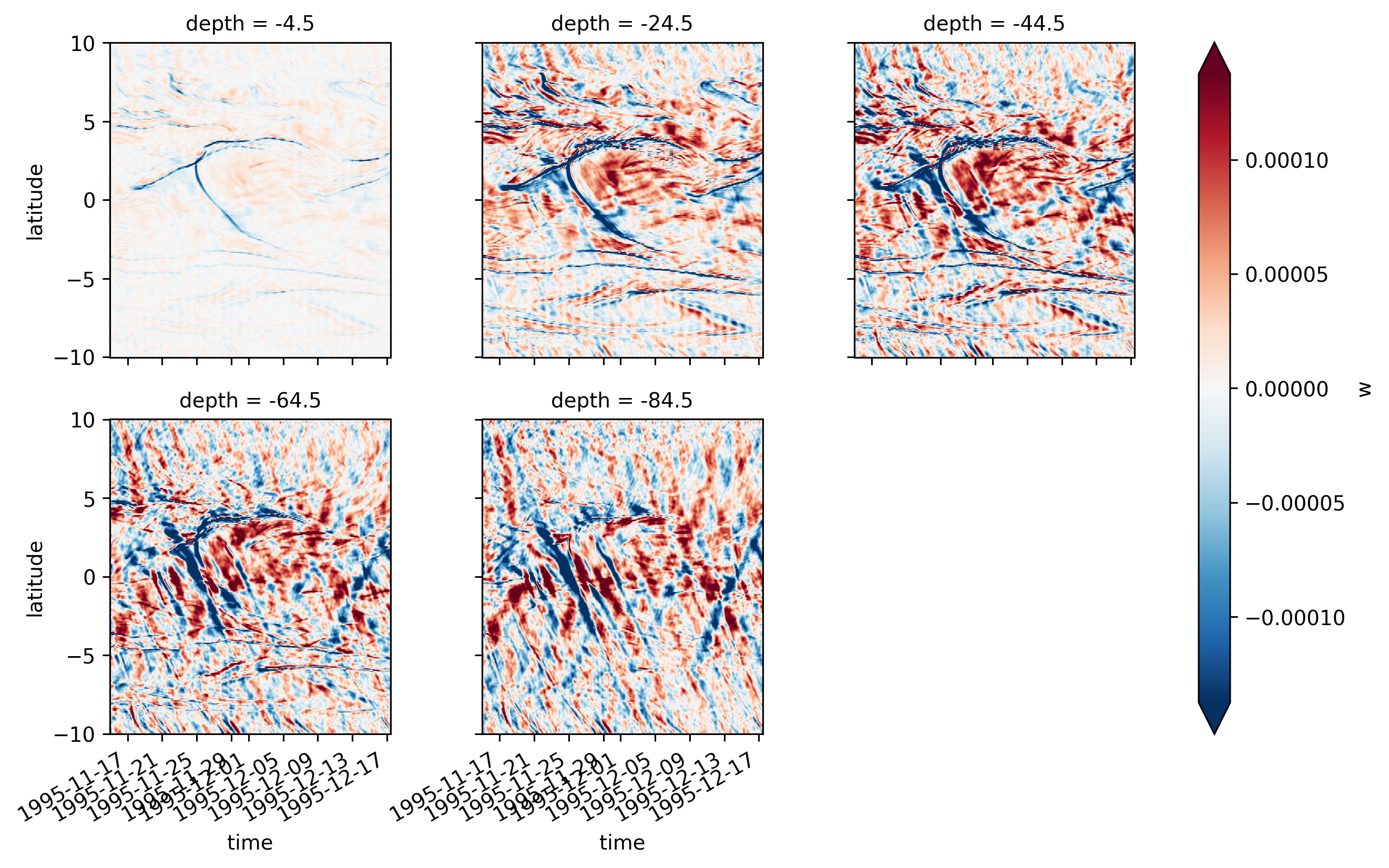
lat-lon top 85m mean#
(central.w.sel(depth=slice(-84.5)).mean("depth").plot(robust=True, x="time"))
<matplotlib.collections.QuadMesh at 0x2b12cc585730>
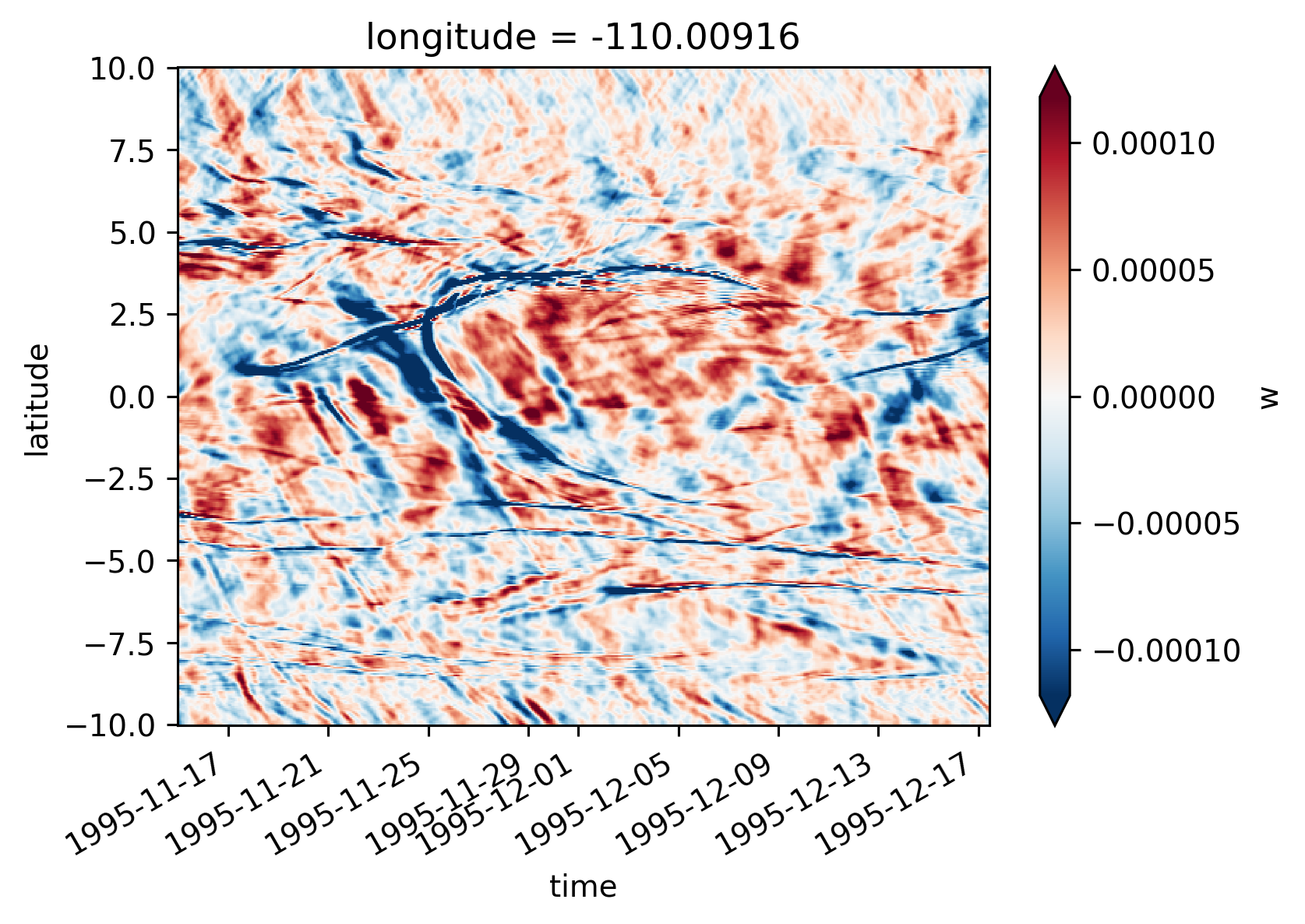
depth-time at lats#
lats = [4, 3, 2, 1, 0, -1]
central.theta.isel(depth=0).plot(robust=True, x="time", cmap=mpl.cm.RdYlBu_r)
[plt.axhline(lat) for lat in lats]
(
central.w.sel(latitude=lats, method="nearest").plot(
col_wrap=2,
col="latitude",
x="time",
robust=True,
cbar_kwargs={"orientation": "horizontal"},
)
)
<xarray.plot.facetgrid.FacetGrid at 0x2b12cea61610>
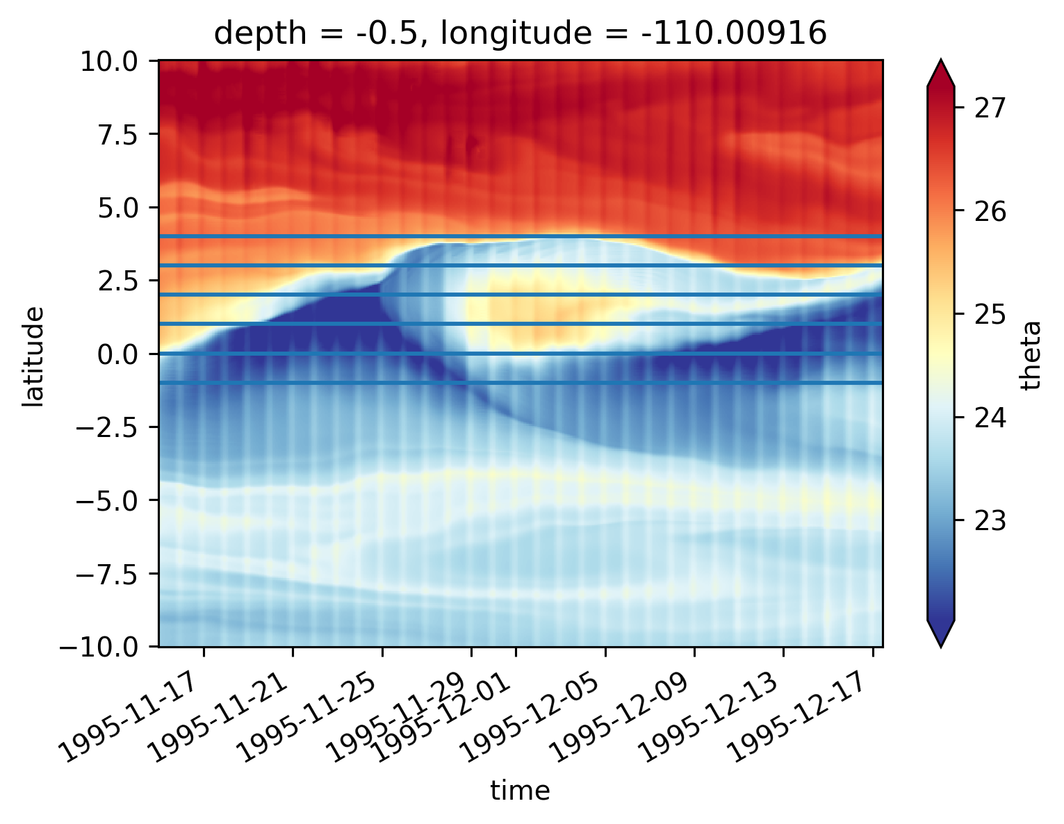
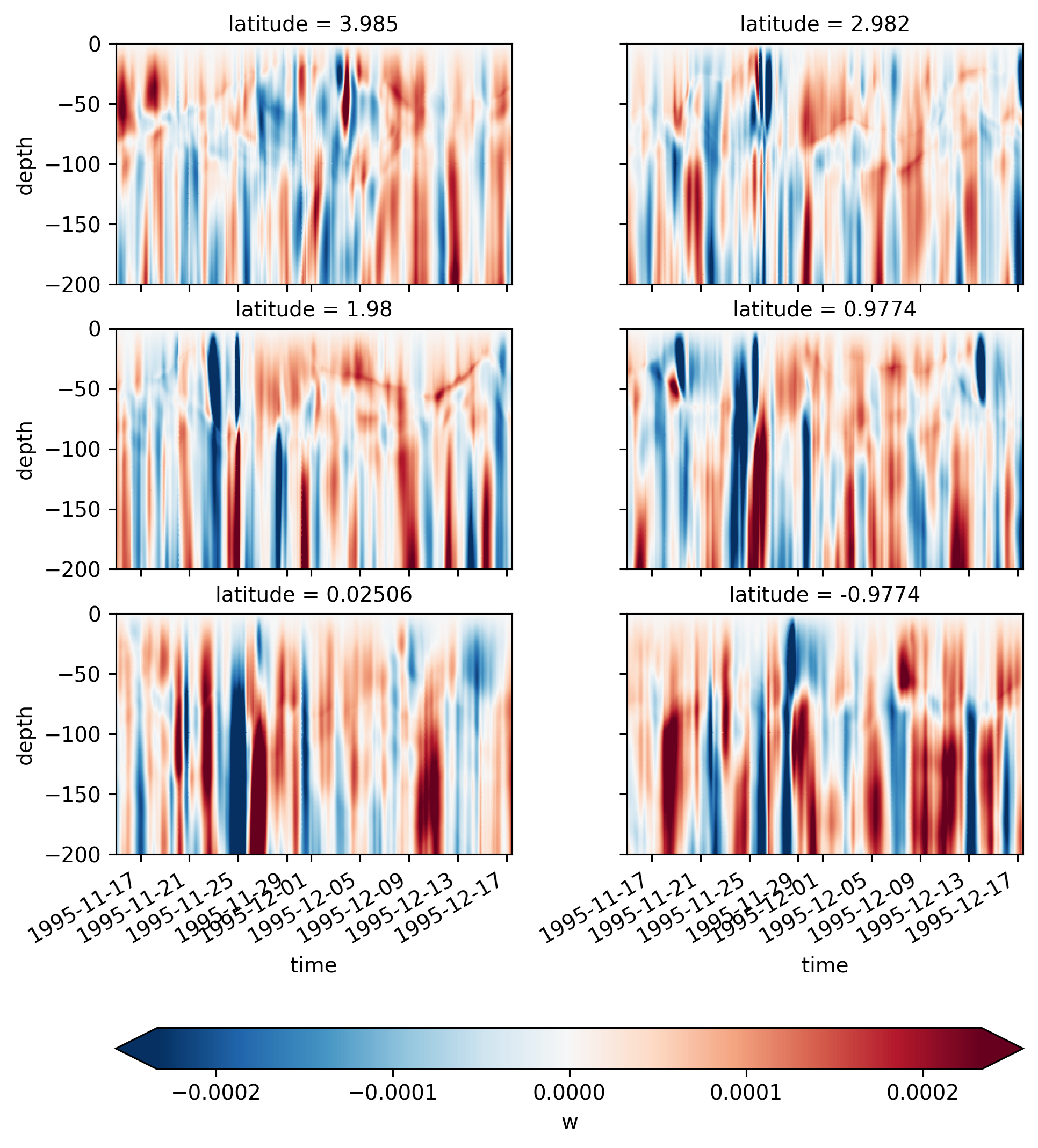
depth-lat at times#
times = [
"1995-11-17",
"1995-11-25",
"1995-11-26",
"1995-11-27",
"1995-12-01",
"1995-12-10",
]
central.theta.isel(depth=0).plot(robust=True, x="time", cmap=mpl.cm.RdYlBu_r)
[plt.axvline(time) for time in times]
fg = central.w.sel(time=[pd.Timestamp(tt) for tt in times]).plot(
y="depth",
row="time",
robust=True,
cbar_kwargs={"orientation": "horizontal"},
xlim=(-5, 5),
)
fg.fig.set_size_inches((8, 6))
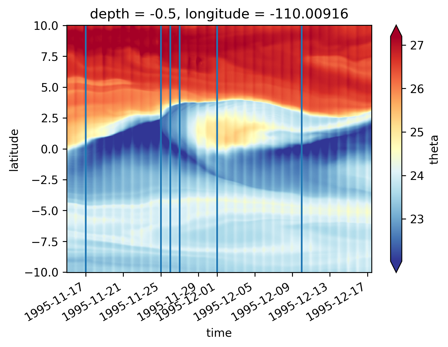
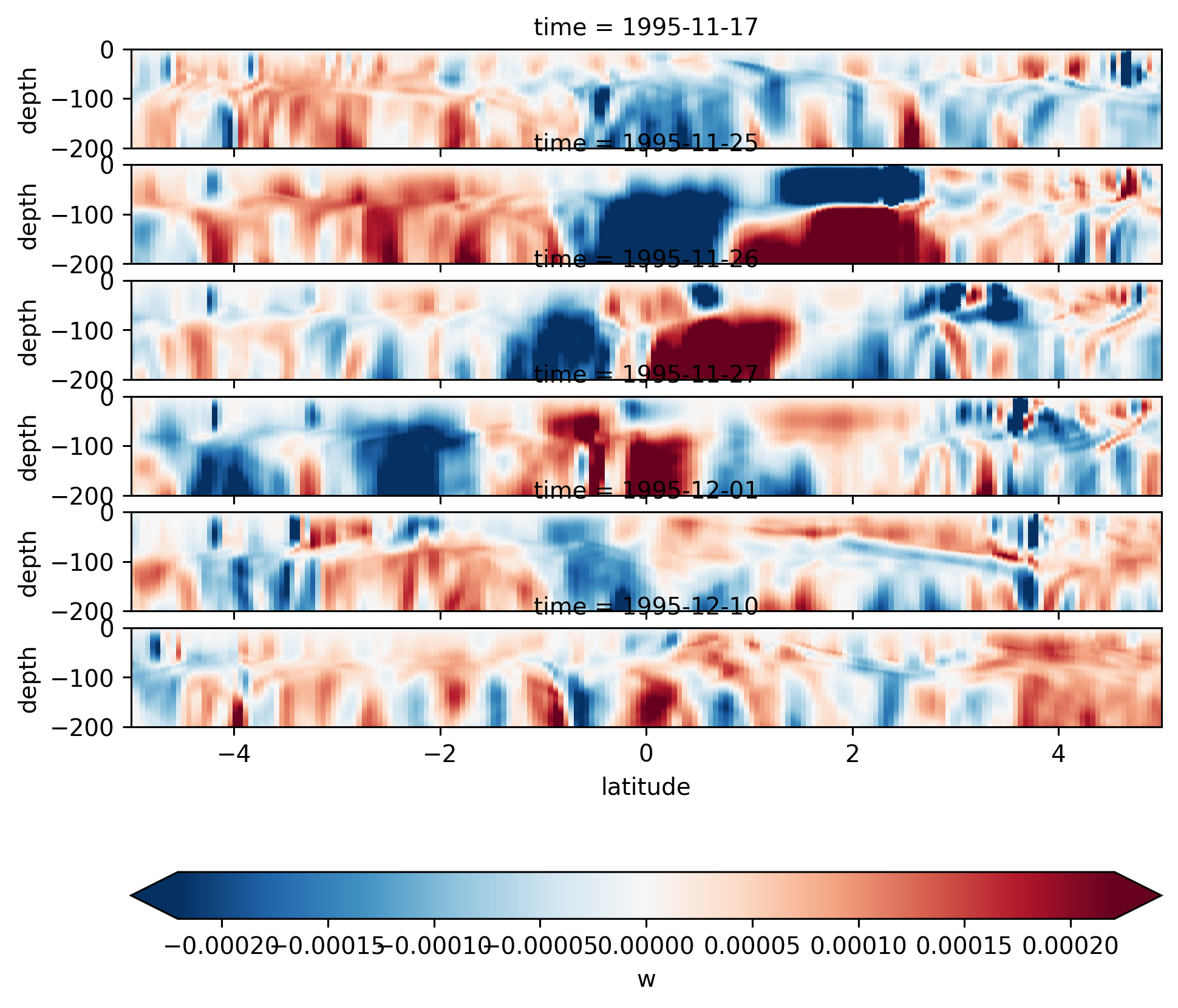
Spectra#
import dcpy
Why is the spectrum white for freq < 2 days?
z = -50
lats = [0, 3, 3.5, 4]
subset = central.w.reindex(latitude=lats, method="nearest").sel(
depth=z, method="nearest"
)
for lat in lats:
dcpy.ts.PlotSpectrum(subset.sel(latitude=lat), label=str(lat), ax=plt.gca())
plt.legend(title="Lat (°N)")
plt.title(f"depth = {z}m")
Text(0.5, 1.0, 'depth = -50m')
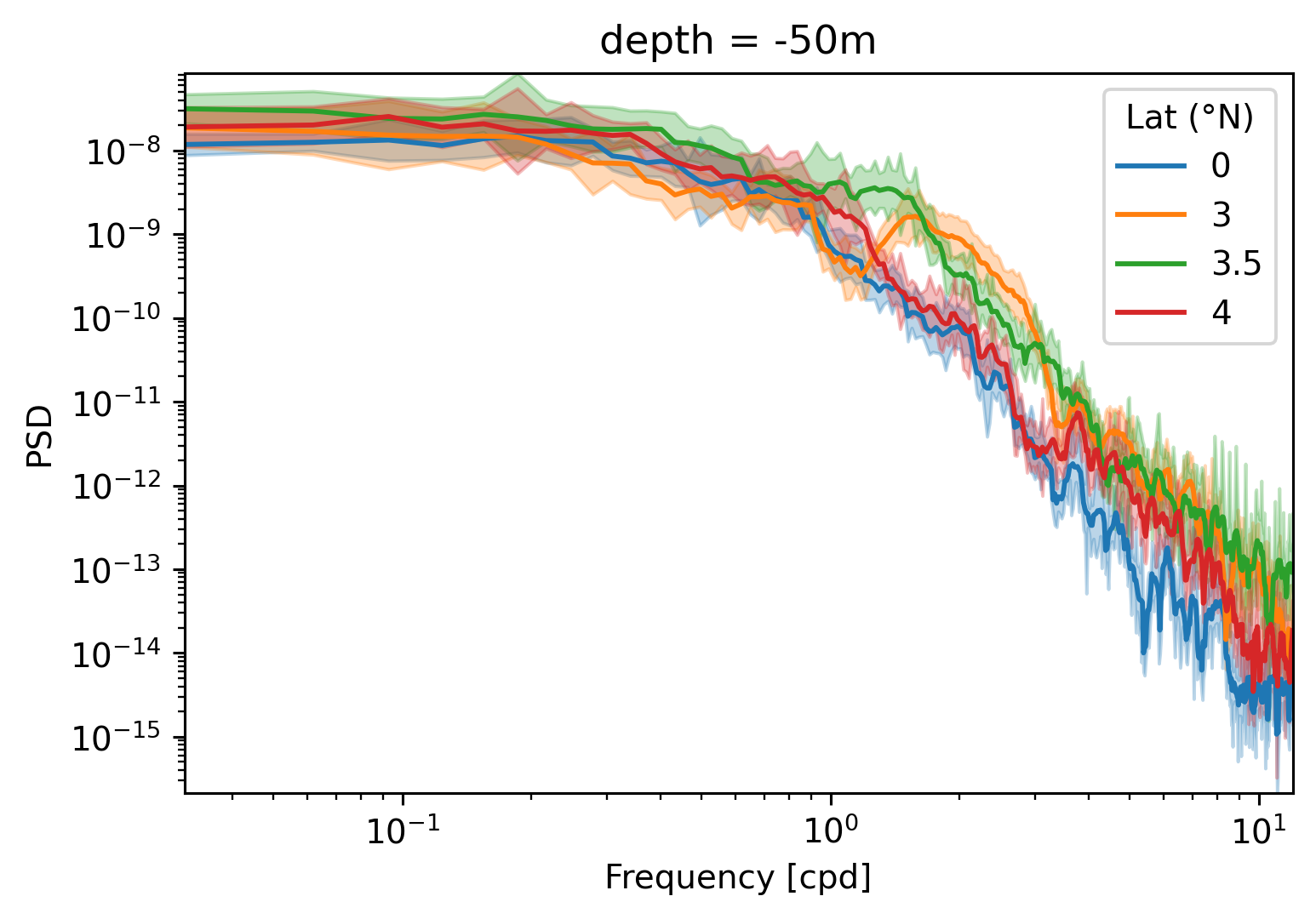
z = -150
subset = central.w.reindex(latitude=lats, method="nearest").sel(
depth=z, method="nearest"
)
for lat in lats:
dcpy.ts.PlotSpectrum(subset.sel(latitude=lat), label=str(lat), ax=plt.gca())
plt.legend(title="Lat (°N)")
plt.title(f"depth = {z}m")
Text(0.5, 1.0, 'depth = -150m')
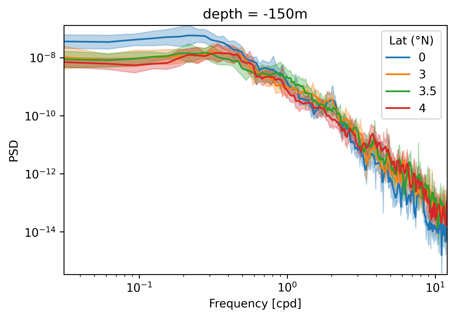
Mixing in T space#
central = central.persist()
plt.rcParams["figure.figsize"] = (8.0, 5.0)
plt.rcParams["figure.dpi"] = 140
def plot_Jq_T(subset):
(-1 * subset.Jq.rolling(depth=2).mean()).compute().differentiate("depth").plot(
x="time", vmin=-100, vmax=100, cmap=mpl.cm.RdBu_r
)
subset.theta.plot.contour(x="time", levels=[20, 21, 22, 23, 23.5, 24])
subset.eucmax.plot.line(x="time", color="k", ls="--")
plt.gca().set_ylim((-125, 0))
plt.gcf().set_size_inches((8, 4))
plot_Jq_T(central.sel(latitude=3.5, method="nearest"))
plt.figure()
plot_Jq_T(central.sel(latitude=0, method="nearest"))
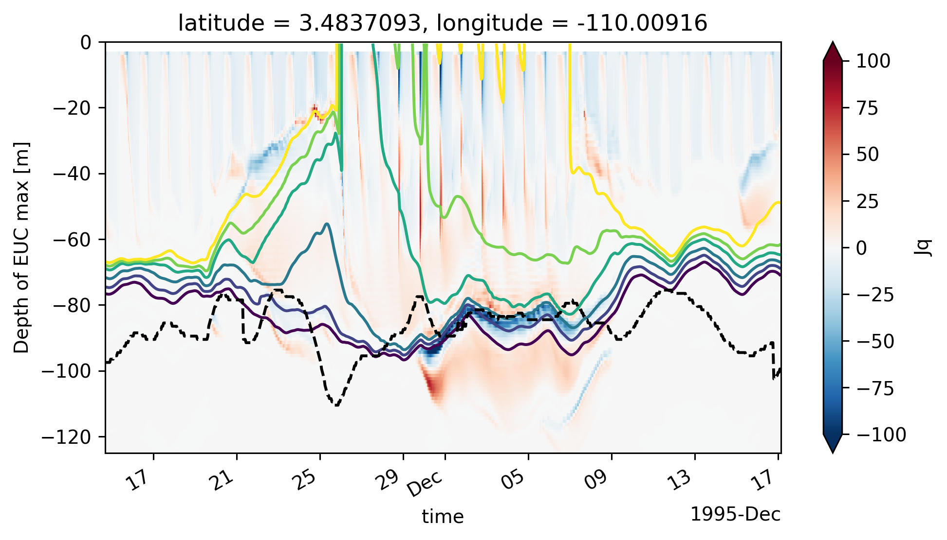
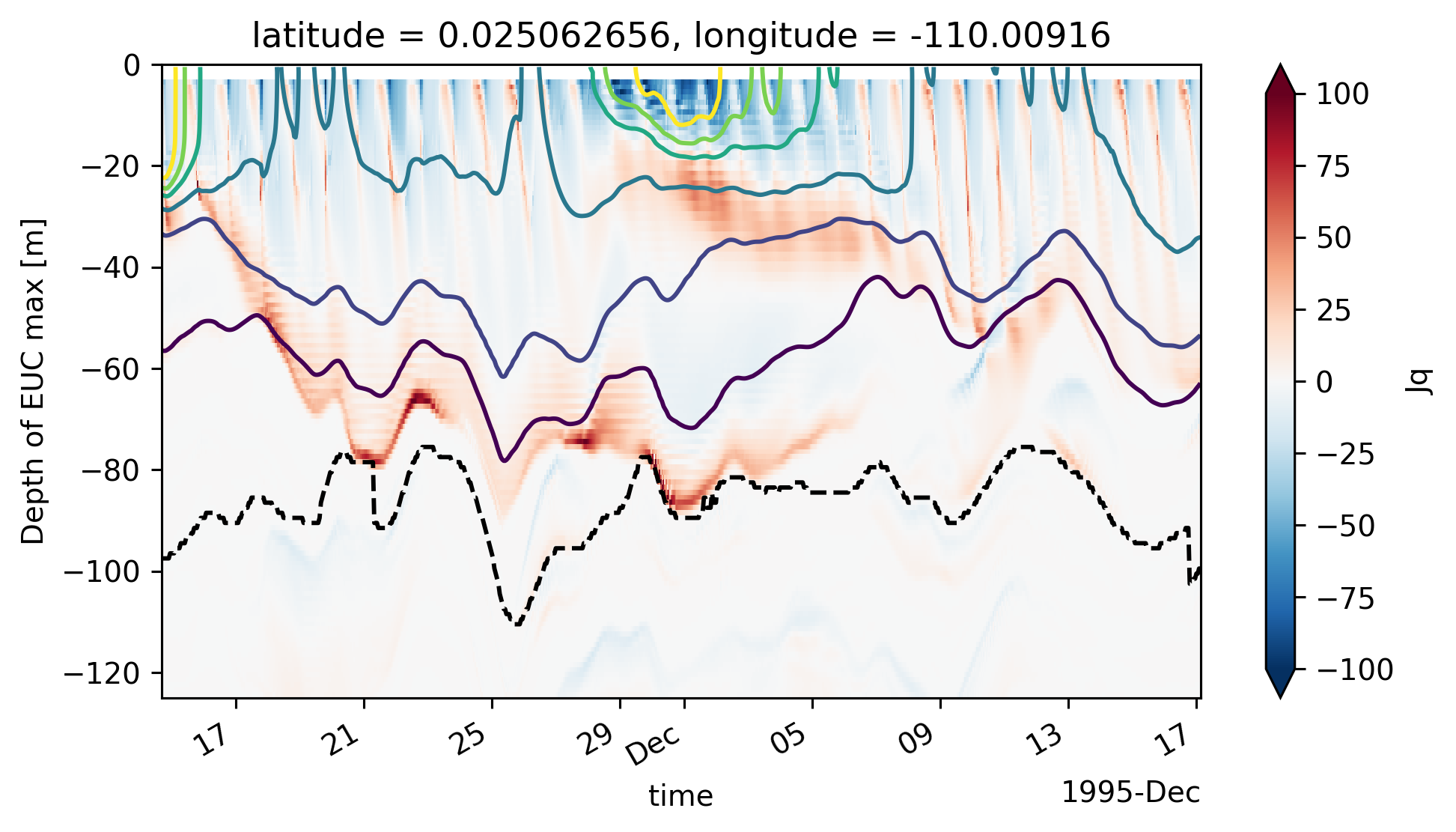
client.cancel(central)