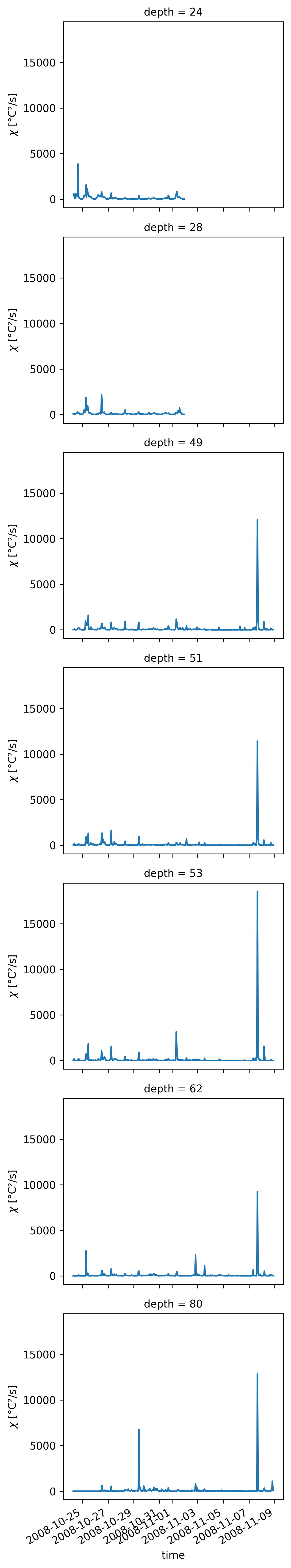
Chameleon heat flux χ vs ε#
I’m confused by disagreements between heat flux calculated from χ or ε.
This notebook studies these differences using chamelon and χpods from EQUIX; and chameleon from TIWE
TODO:
calculate gradients using sorted profiles; this bumps up Jq by a factor of 2!
Sasha’s dTdz is calculated using θ sorted by θ, and N2 is calculated using σ sorted by σ
Sasha’s χpod N2 = gα dTdz with α calculated using S=34
Seems very sensitive to low gradient locations
Figure out what level to filter χ, ε at: 1e-2? 1e-5 in jims multiprofv2.m
Add values for sensor 1, sensor2 to χpod datasets
Add Jq_ε for χpods
Try with TH or TIWE
Need TIWE ADCP
Show code cell content
%load_ext watermark
%load_ext snakeviz
%matplotlib inline


import glob
import os

import cf_xarray as cfxr
import datatree
import dcpy
import distributed
import flox.xarray
import hvplot.xarray
import matplotlib as mpl
import matplotlib.pyplot as plt
import numpy as np
import xarray as xr
from dcpy.oceans import read_osu_microstructure_mat, thorpesort
from IPython.display import Image

# import eddydiff as ed
import pump

xr.set_options(keep_attrs=True)
mpl.rcParams["figure.dpi"] = 140

%watermark -iv
cf_xarray  : 0.7.0
dcpy       : 0.2.1.dev4+g05012cc.d20220325
pump       : 0.1
matplotlib : 3.5.1
xarray     : 2022.3.0
datatree   : 0.0.2.dev1+g2503606.d20220325
distributed: 2022.3.0
flox       : 0.4.1.dev11+gd895625.d20220401
hvplot     : 0.7.3
numpy      : 1.21.5
def Jq(x, *, min_dTdz):
    j = (
        (
            1025
            * 4000
            * x.chi.where(x.chi < 2e-2)
            / 2
            / x.dTdz.where(np.abs(x.dTdz) > min_dTdz)
        )
        .rolling(depth=5, center=True)
        .mean()
    )
    j.attrs["long_name"] = "$J_q^χ$"
    j.attrs["units"] = "W/m^2"
    return j
Read datasets#
EQUIX Chameleon#
On masking#
There are some masks applied in XXX.m, I think the dataset I have has those masks applied.
# badmask = (cham.VARAZ > 0.01) & (np.log10(cham.AZ2) > -4.5) & (cham.eps > 1e-4)
# cham = cham.where(~badmask)
On sorting and calculating gradients#
I’m trying to replicate Sasha’s dT/dz
Sasha’s dT/dz looks like he’s sorted \(T\) by \(T\), instead of \(ρ\), but I still have trouble replicating. Note he has no negative values.
cali_eq08.m is useful. SIGMA_ORDER and THETA_ORDER are thorpesorted using calc_order
% calculate SIGMA_ORDER
inds=calc_order('sigma','P');
% calculate THETA_ORDER
inds=calc_order('theta','P');

% calculate the mean temperature gradient on small scales:
cal.DTDZ=diff(cal.THETA_ORDER)./diff(cal.P);
cal.DTDZ(length(cal.DTDZ)+1)=cal.DTDZ(length(cal.DTDZ));
head.irep.DTDZ=1;

% calculate the mean density gradient on small scales:
cal.DRHODZ=diff(cal.SIGMA_ORDER)./diff(cal.P);
cal.DRHODZ(length(cal.DRHODZ)+1)=cal.DRHODZ(length(cal.DRHODZ));
head.irep.DRHODZ=1;
g=9.81;
cal.SIGMA=cal.SIGMA-1000;
cal.SIGMA_ORDER=cal.SIGMA_ORDER-1000;
rhoav=mean(cal.SIGMA(1:1:length(cal.SIGMA)-1))+1000;

cal.N2=(g/rhoav).*diff(cal.SIGMA_ORDER)./diff(cal.P);
cal.N2(length(cal.N2)+1)=cal.N2(length(cal.N2));
This confirms that THETA is sorted by THETA and SIGMA by SIGMA. A simple diff is used and the last value is repeated at the end.
Some deglitching of N2 happens in sum_eq08.m
cham = xr.load_dataset(os.path.expanduser("~/datasets/microstructure/osu/equix.nc"))

cham["rhoav"] = cham.pden.mean().data + 1000
cham["dTdz"] *= -1

theta_old = cham.theta.copy(deep=True)
cham["depth"] = cham.depth.astype(float)
cham["sortTbyT"] = thorpesort(cham.theta, cham.theta, ascending=False)
cham["sortT"] = thorpesort(cham.theta, cham.pden, ascending=True)
cham["NT2"] = (
    -9.81
    * dcpy.eos.alpha(
        34 * xr.ones_like(cham.theta), cham.theta, cham.pres.broadcast_like(cham.theta)
    )
    * cham.dTdz
)

chamρ = thorpesort(cham.drop("pres"), "pden", core_dim="depth")
chamρ["pres"] = cham.pres
chamρ["dTdz"] = -chamρ.theta.diff("depth", label="lower")
chamρ["N2"] = 9.81 / cham.rhoav * chamρ.pden.diff("depth", label="lower")
chamρ["NT2"] = (
    9.81
    * dcpy.eos.alpha(
        34 * xr.ones_like(chamρ.theta),
        chamρ.theta,
        chamρ.pres.broadcast_like(chamρ.theta),
    )
    * chamρ.dTdz
)

chamT = thorpesort(cham.drop("pres"), "theta", core_dim="depth", ascending=False)
chamT["pres"] = cham.pres
chamT["dTdz"] = -chamT.theta.diff("depth", label="lower")
chamT["N2"] = 9.81 / cham.rhoav * chamT.pden.diff("depth", label="lower")
chamT["NT2"] = (
    9.81
    * dcpy.eos.alpha(
        34 * xr.ones_like(chamT.theta),
        chamT.theta,
        chamT.pres.broadcast_like(chamT.theta),
    )
    * chamT.dTdz
)
cham
OMP: Info #273: omp_set_nested routine deprecated, please use omp_set_max_active_levels instead.
<xarray.Dataset>
Dimensions:          (depth: 200, time: 2624, zeuc: 80)
Coordinates:
  * depth            (depth) float64 1.0 2.0 3.0 4.0 ... 197.0 198.0 199.0 200.0
    lon              (time) float64 -139.9 -139.9 -139.9 ... -139.9 -139.9
    lat              (time) float64 0.06246 0.0622 0.06263 ... 0.06317 0.06341
  * time             (time) datetime64[ns] 2008-10-24T20:36:23 ... 2008-11-08...
  * zeuc             (zeuc) float64 -200.0 -195.0 -190.0 ... 185.0 190.0 195.0
Data variables: (12/49)
    pmax             (time) float64 205.9 199.0 202.0 ... 202.0 221.1 203.9
    castnumber       (time) uint16 16 17 18 19 20 ... 2664 2665 2666 2667 2668
    AX_TILT          (depth, time) float64 9.642 -48.16 nan ... 4.232 1.28
    AY_TILT          (depth, time) float64 14.52 11.51 nan ... -2.121 0.05032
    AZ2              (depth, time) float64 0.04277 1.537e-05 ... 3.208e-06
    C                (depth, time) float64 5.244 5.291 nan ... 4.135 4.137 4.164
    ...               ...
    count_dJdz_euc   (time, zeuc) int64 0 0 0 0 0 0 0 0 0 ... 0 0 0 0 0 0 0 0 0
    count_dTdt_euc   (time, zeuc) int64 0 0 0 0 0 0 0 0 0 ... 0 0 0 0 0 0 0 0 0
    count_u_euc      (time, zeuc) int64 0 0 0 0 0 0 0 0 0 ... 0 0 0 0 0 0 0 0 0
    count_depth_euc  (time, zeuc) int64 0 0 0 0 0 0 0 0 0 ... 0 0 0 0 0 0 0 0 0
    rhoav            float64 1.025e+03
    NT2              (depth, time) float64 nan nan nan ... -0.0001089 -0.000102
Attributes:
    starttime:  ['Time:20:34:29 298   ' 'Time:20:42:18 298   ' 'Time:20:52:14...
endtime: ['Time:20:38:29 298 ' 'Time:20:46:29 298 ' 'Time:20:56:29...Comparing gradients#
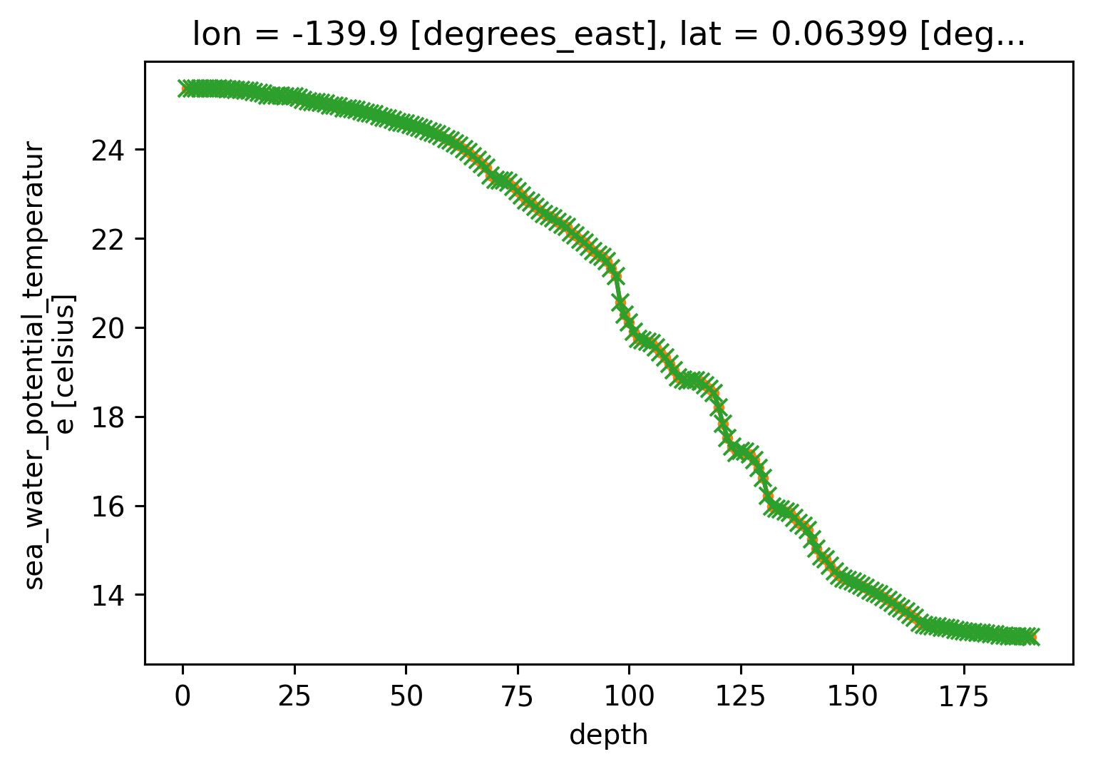
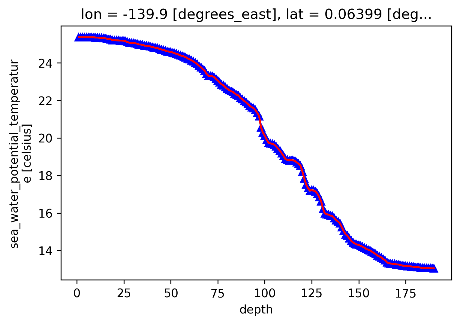
profile = cham.isel(time=200)
# 1m spacing so a simple diff is the gradient...
profile.theta.diff("depth", label="lower").plot(aspect=4, size=5, label="dtheta/dz")
profile.sortT.diff("depth", label="lower").plot(label="d/dz sorted by ρ")
profile.sortTbyT.diff("depth", label="lower").plot(label="d/dz sorted by T")
# cham5m.T.isel(time=150).diff("depth").plot()
(-1 * profile.dTdz).plot(color="k", label="Sasha")
dcpy.plots.liney(0)
plt.legend()
<matplotlib.legend.Legend at 0x7fabc98c5910>

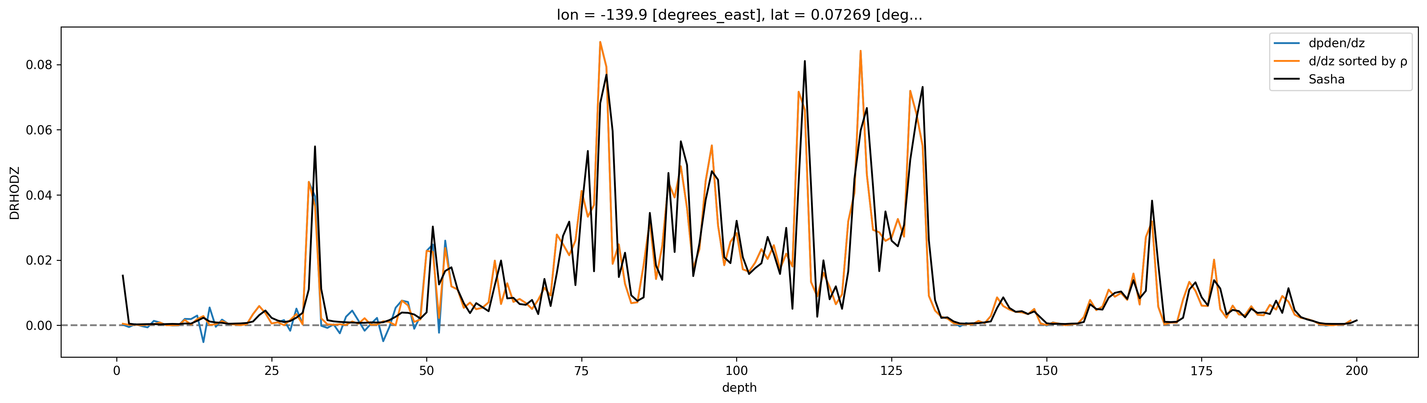
profile = cham.isel(time=200)
# 1m spacing so a simple diff is the gradient...
profile.pden.diff("depth", label="lower").plot(aspect=4, size=5, label="dpden/dz")
chamρ.isel(time=200).pden.diff("depth", label="lower").plot(label="d/dz sorted by ρ")
# cham5m.T.isel(time=150).diff("depth").plot()
profile.DRHODZ.plot(color="k", label="Sasha")
dcpy.plots.liney(0)
plt.legend()
<matplotlib.legend.Legend at 0x7fab509d7be0>
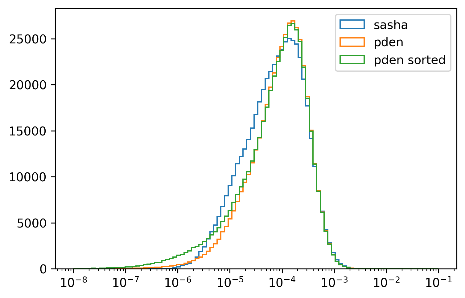
for da in [
    cham.N2,
    (9.81 / cham.rhoav * cham.pden.diff("depth") / cham.pres.diff("depth")),
    (9.81 / cham.rhoav * chamρ.pden.diff("depth") / cham.pres.diff("depth")),
]:
    da.plot.hist(
        yscale="linear", bins=np.logspace(-8, -1, 100), xscale="log", histtype="step"
    )

plt.legend(["sasha", "pden", "pden sorted"])
<matplotlib.legend.Legend at 0x7fab8885db80>
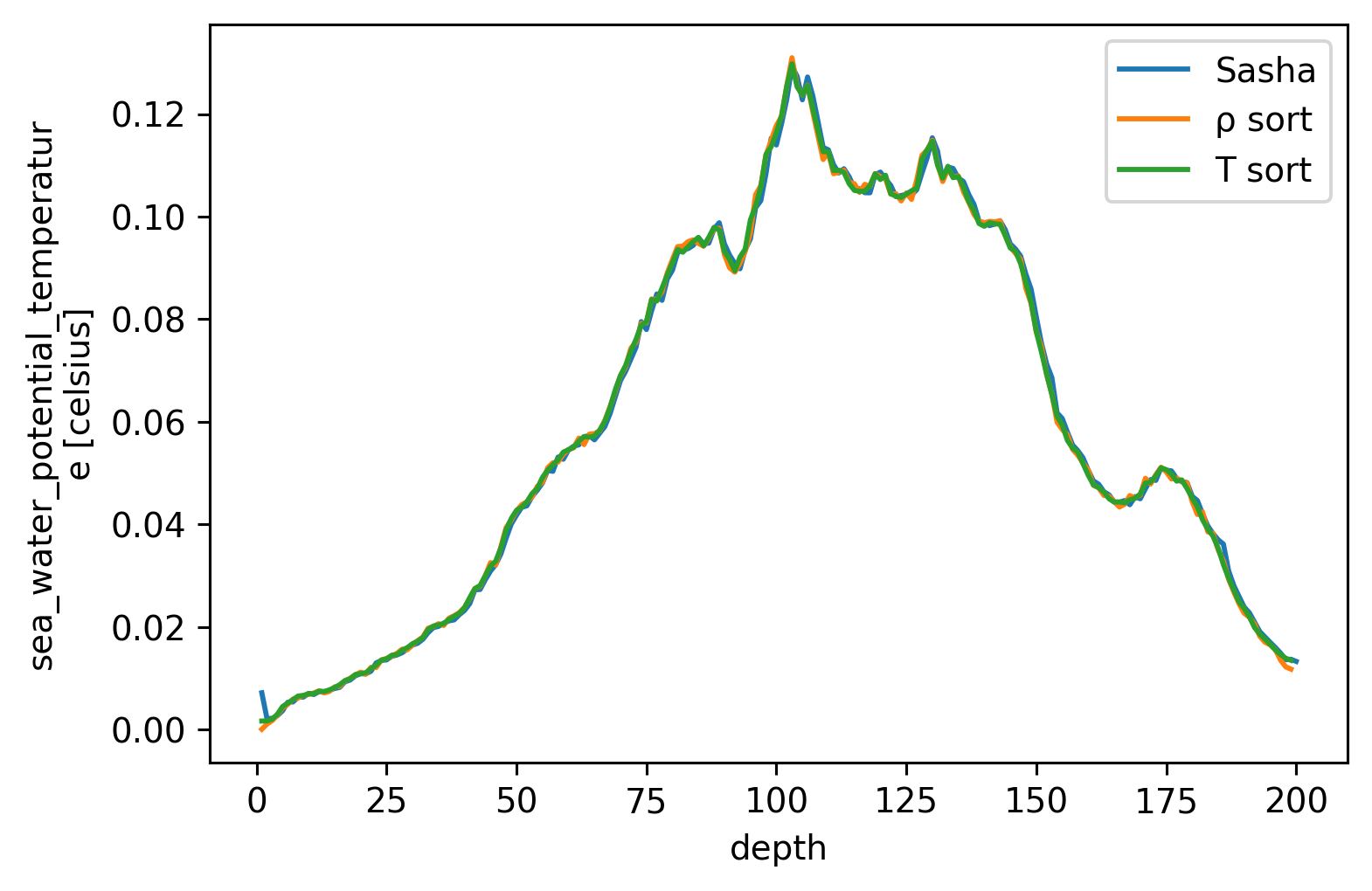
cham.dTdz.mean("time").plot(label="Sasha")
chamρ.dTdz.mean("time").plot(label="ρ sort")
chamT.dTdz.mean("time").plot(label="T sort")
plt.legend()
<matplotlib.legend.Legend at 0x7fab8885dee0>
EQUIX χpods#
tao = xr.open_dataset(
    os.path.expanduser("~/work/datasets/microstructure/osu/equix/hourly_tao.nc")
)
iop = xr.open_dataset(
    os.path.expanduser("~/datasets/microstructure/osu/equix/hourly_iop.nc")
)
eop = xr.open_dataset(
    os.path.expanduser("~/datasets/microstructure/osu/equix/hourly_eop.nc")
)
tao_iop = xr.open_dataset(
    os.path.expanduser("~/datasets/microstructure/osu/equix/hourly_tao_iop.nc")
)

for suffix in ["1", "2"]:
    tao_iop["NT2" + suffix] = (
        9.81
        * dcpy.eos.alpha(
            34 * np.ones_like(tao_iop["T1"]),
            tao_iop["T" + suffix],
            tao_iop.depth.broadcast_like(tao_iop.T1),
        )
        * tao_iop[f"dT{suffix}dz"]
    )
tao_iop["NT2"] = (
    9.81
    * dcpy.eos.alpha(34 * xr.ones_like(tao_iop.T1), tao_iop.T1, tao_iop.depth)
    * tao_iop.dTdz
)
iop["NT2"] = (
    9.81 * dcpy.eos.alpha(34 * xr.ones_like(iop.theta), iop.theta, iop.depth) * iop.dTdz
)

iop["Jq_eps"] = 4200 * 1025 * 0.2 * iop.eps / iop.NT2.where(iop.NT2 > 5e-6) * iop.dTdz
tao_iop["Jq_eps"] = (
    4200
    * 1025
    * 0.2
    * tao_iop.eps
    / tao_iop.NT2.where(tao_iop.NT2 > 5e-6)
    * tao_iop.dTdz
)

Tbins = np.hstack(
    [np.arange(18, 22, 1), np.arange(22, 25, 0.5), np.arange(25, 26.1, 0.25)]
)
# mask = np.ones_like(cham.dTdz, dtype=bool)
mask = (np.abs(cham.dTdz) > 1e-3) & (cham.N2 > 1e-5)
(cham.chi / 2 / cham.dTdz.where(mask) ** 2).mean("time").plot(
    y="depth", xscale="log", yincrease=False
)
(0.2 * cham.eps / cham.N2.where(mask)).mean("time").plot(
    y="depth", xscale="log", yincrease=False, ylim=(100, 25)
)
[<matplotlib.lines.Line2D at 0x7faba97f7070>]
TIWE chameleon#
tiwe = xr.load_dataset(os.path.expanduser("~/datasets/microstructure/osu/tiwe.nc")).sel(
    depth=slice(200)
)
tiwe["rhoav"] = tiwe.pden.mean() + 1000

tiweρ = thorpesort(tiwe.drop("pres"), "pden", core_dim="depth")
tiweρ["dTdz"] = -1 * tiweρ.theta.diff("depth", label="lower")
tiweρ["N2"] = 9.81 / tiweρ.rhoav * tiweρ.pden.diff("depth", label="lower")
tiweρ["pres"] = tiwe.pres
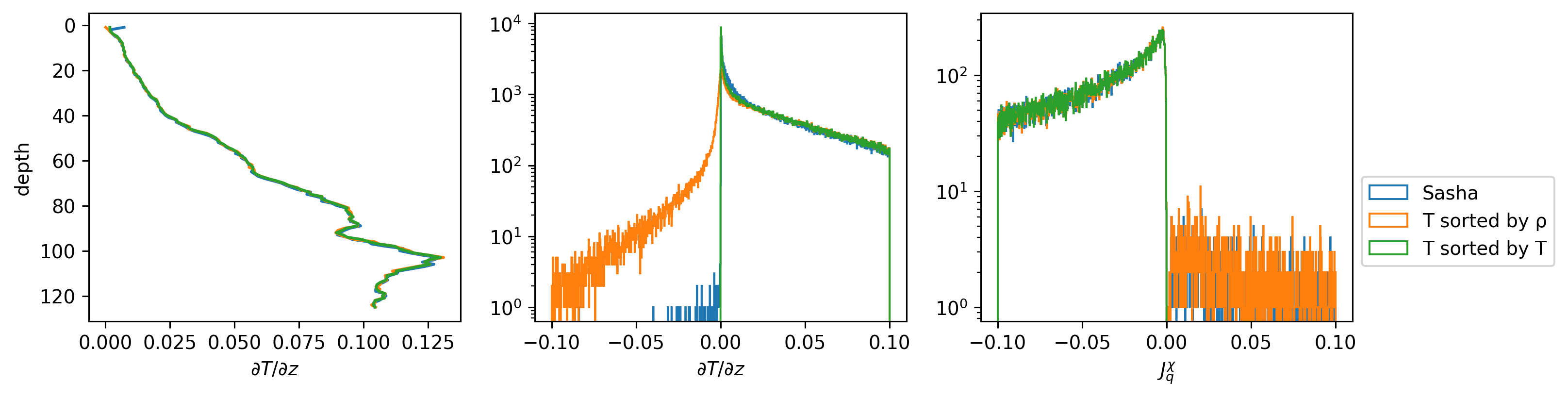
Different Jq calculations#
f, ax = plt.subplots(1, 3)
f.set_size_inches((12, 3))

cham.dTdz.sel(depth=slice(125)).mean("time").cf.plot(ax=ax[0])
chamρ.dTdz.sel(depth=slice(125)).mean("time").cf.plot(ax=ax[0])
chamT.dTdz.sel(depth=slice(125)).mean("time").cf.plot(ax=ax[0])

ax[0].set_xlabel("$∂T/∂z$")

_, bins, _ = cham.dTdz.sel(depth=slice(125)).plot.hist(
    histtype="step", bins=np.linspace(-0.1, 0.1, 1000), ax=ax[1], label="Sasha"
)
chamρ.dTdz.sel(depth=slice(125)).plot.hist(
    histtype="step", bins=bins, yscale="log", ax=ax[1], label="T sorted by ρ"
)
chamT.dTdz.sel(depth=slice(125)).plot.hist(
    histtype="step",
    bins=bins,
    yscale="log",
    ax=ax[1],
    label="T sorted by T",
)
ax[1].set_xlabel("$∂T/∂z$")


def Jq_(x, Tname):
    dTdz = x[Tname].differentiate("depth")
    return x.rhoav * 4000 * x.chi.where(x.chi < 1e-2) / 2 / dTdz


_, bins, _ = (
    Jq_(cham, "T")
    .sel(depth=slice(125))
    .plot.hist(
        histtype="step", bins=np.linspace(-0.1, 0.1, 1000), ax=ax[2], label="Sasha"
    )
)
Jq_(cham, "sortT").sel(depth=slice(125)).plot.hist(
    histtype="step", bins=bins, yscale="log", ax=ax[2], label="T sorted by ρ"
)
Jq_(cham, "sortTbyT").sel(depth=slice(125)).plot.hist(
    histtype="step",
    bins=bins,
    yscale="log",
    ax=ax[2],
    label="T sorted by T",
)

ax[-1].set_xlabel("$J_q^χ$")
ax[-1].legend(bbox_to_anchor=(1.0, 0.5))
<matplotlib.legend.Legend at 0x7fab581a3d30>
profile = cham.isel(time=200)
# profile.N2.plot()
(profile.DRHODZ).plot()
(thorpesort(profile.pden, profile.pden).diff("depth")).plot()
[<matplotlib.lines.Line2D at 0x7fab55a9edf0>]
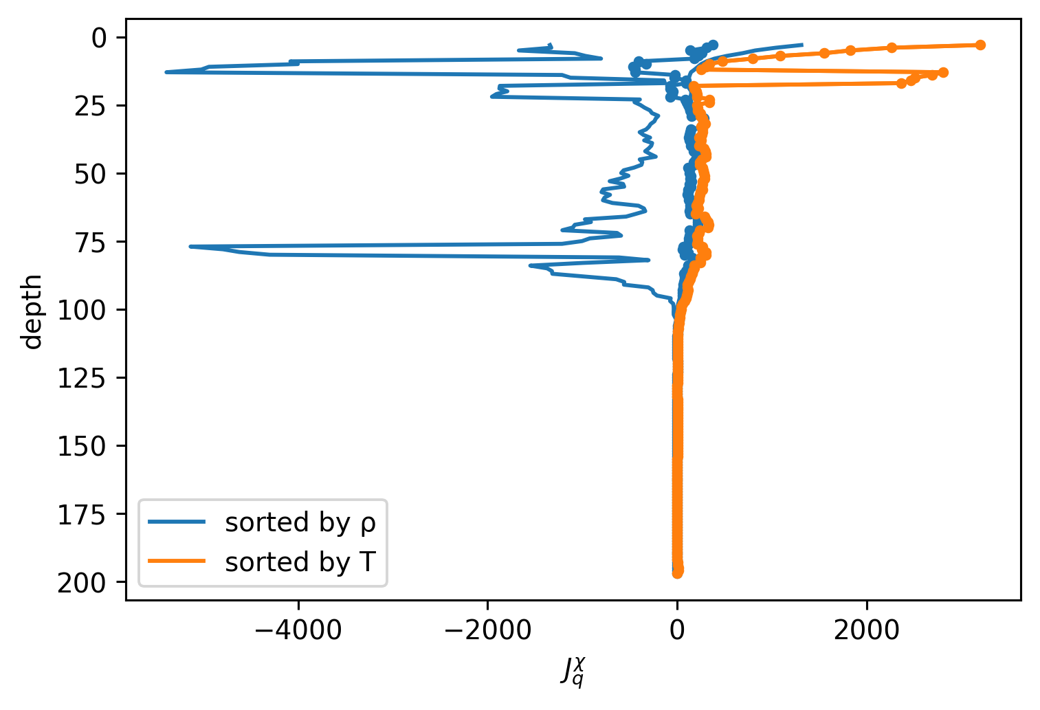
def plot(c, name):
    j = Jq(c, min_dTdz=1e-3)
    hdl = j.where(j < 0).mean("time").plot(y="depth", label=name)
    j.where(j > 0).mean("time").plot(
        color=hdl[0].get_color(), y="depth", yincrease=False
    )
    j.mean("time").plot(
        marker=".", color=hdl[0].get_color(), y="depth", yincrease=False
    )


plot(chamρ, "sorted by ρ")
plot(chamT, "sorted by T")
plt.legend()
plt.xlabel("$J_q^χ$")
Text(0.5, 0, '$J_q^χ$')
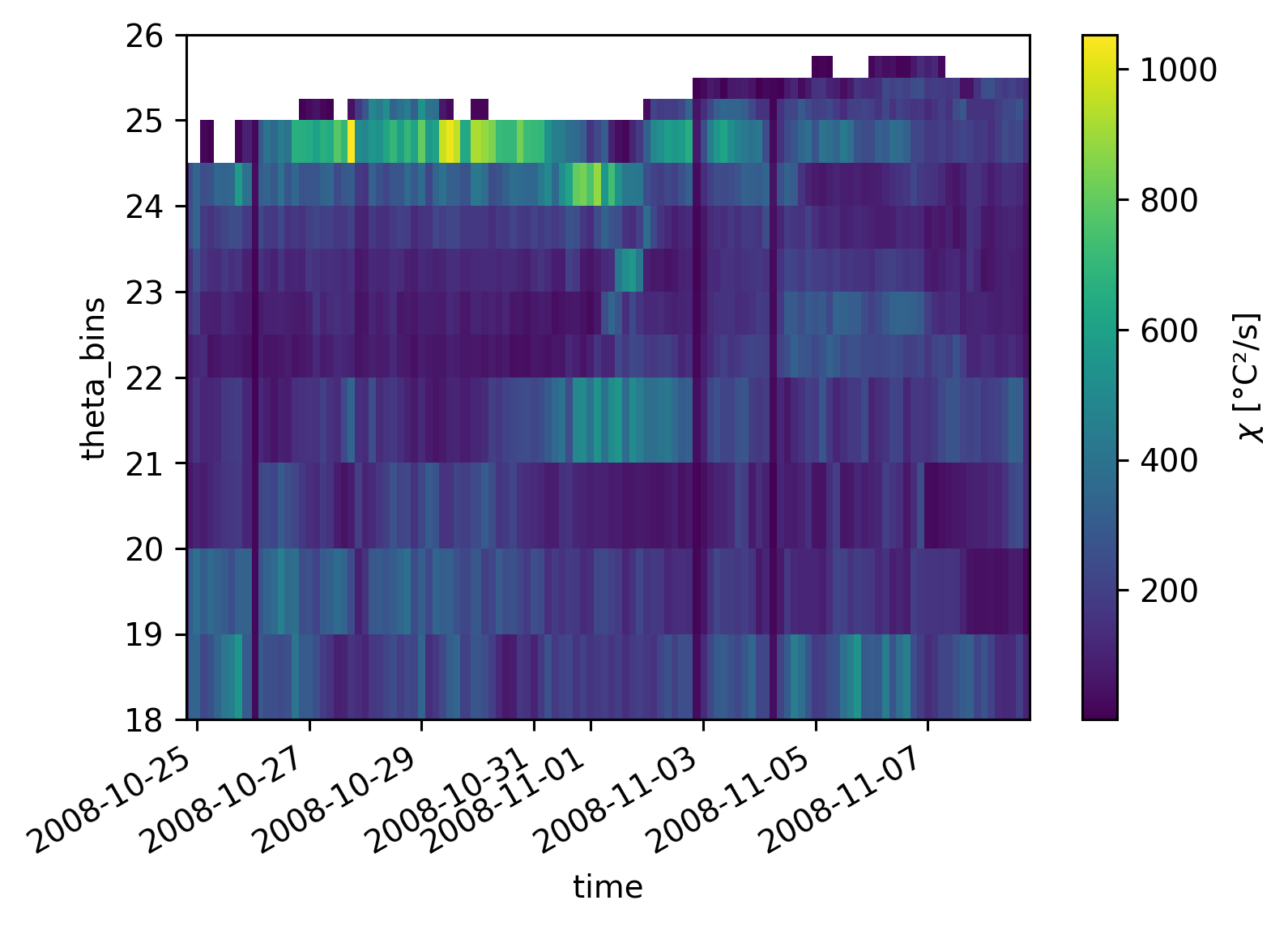
Averaging in temperature space#
# xr.set_options(use_numpy_groupies=False)
# cham_legacy = pump.tspace.regrid_chameleon(
# These thresholds make a big difference! but really it's a very small number of points
#    cham.where((cham.chi < 1e-2) & (cham.eps < 1e-5))
#    .sel(depth=slice(156))
#    .where(cham.depth > cham.mld + 5)
#    .isel(time=slice(24 * 6)),
#    time_freq="3H",
#    bins=bins,
#    trim_mld=False,
# )
f, ax = plt.subplots(1, 2, sharey=True)
cham_legacy.chi.mean("time").plot(ax=ax[0], y="theta_c")
cham_npg.chi.mean("time").plot(ax=ax[0], y="theta_c")

(cham_legacy.nobs - cham_npg.nobs).plot(ax=ax[1], y="theta_bins", cmap=mpl.cm.Reds)
# xr.set_options(use_flox=True)
cham_npg = pump.tspace.regrid_chameleon(
    # These thresholds make a big difference! but really it's a very small number of points
    cham.where((cham.chi < 1e-2))
    .sel(depth=slice(156))
    .where(cham.depth > cham.mld + 5),
    # .isel(time=slice(24 * 6)),
    time_freq="3H",
    bins=Tbins,
    trim_mld=False,
)
cham_Tspace = cham_npg
cham_Tmean = cham_Tspace.mean("time")
cham_Tmean.coords["z_c"] = cham_Tspace.z_c.mean("time")
%matplotlib inline
mpl.rcParams["figure.dpi"] = 140
cham_Tspace.nobs.plot(x="time")
plt.figure()
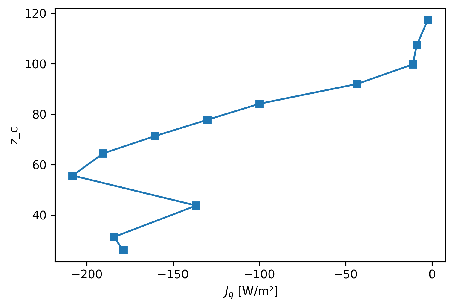
cham_Tmean.Jq.plot(y="z_c", marker="s", yincrease=True)
[<matplotlib.lines.Line2D at 0x7fdca55ae190>]
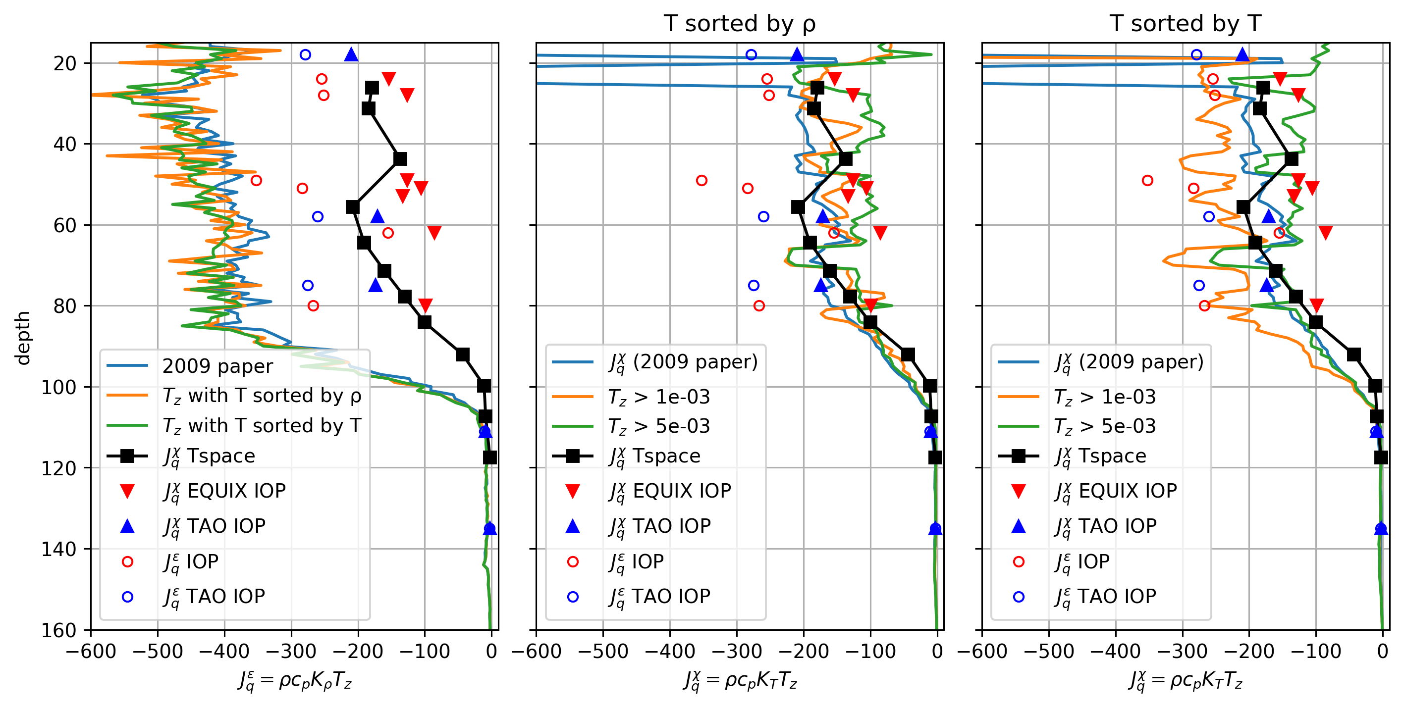
\(J_q^ε\) vs \(J_q^χ\)#
Define
\begin{align*} J_q^χ &= ρ c_p K_T T_z = ρ c_p \frac{χ/2}{T_z^2} T_z \ J_q^ε &= ρ c_p K_ρ T_z = ρ c_p \frac{Γε}{N²} T_z \end{align*}
Compare many Jq estimates: \(J_q^χ\) and \(J_q^ε\) from χpod, chameleon
f, ax = plt.subplots(1, 3, sharex=True, sharey=True, constrained_layout=True)
f.set_size_inches((10, 5))

N2rho = 9.81 / 1025 * cham.pden.differentiate("depth")
N2sort = 9.81 / 1025 * thorpesort(cham.pden, cham.pden).differentiate("depth")
for cham_, label in zip(
    [cham, chamρ, chamT],
    ["2009 paper", "$T_z$ with T sorted by ρ", "$T_z$ with T sorted by T"],
):
    (1025 * 4000 * 0.2 * cham.eps / cham.N2.where(cham.N2 > 5e-6) * cham_.dTdz).mean(
        "time"
    ).plot(
        y="depth",
        yincrease=False,
        # color="k",
        label=label,
        ax=ax[0],
    )
ax[0].set_xlabel("$J_q^ε = ρ c_p K_ρ T_z$")


for cham_, axx in zip([chamρ, chamT], ax[1:]):
    Jq(cham, min_dTdz=1e-10).mean("time").plot(
        y="depth",
        yincrease=False,
        label="$J_q^χ$ (2009 paper)",
        ax=axx,
    )
    for min_dTdz in [1e-3, 5e-3]:
        Jq(cham_, min_dTdz=min_dTdz).mean("time").plot(
            y="depth",
            yincrease=False,
            label=f"$T_z$ > {min_dTdz:.0e}",
            ax=axx,
        )
    axx.set_xlabel("$J_q^χ = ρ c_p K_T T_z$")

for axx in ax:
    cham_Tmean.Jq.plot(
        y="z_c",
        marker="s",
        color="k",
        label="$J_q^χ$ Tspace",
        ax=axx,
        _labels=False,
    )
    (-1 * iop.Jq).mean("time").plot(
        y="depth",
        marker="v",
        ls="none",
        label="$J_q^χ$ EQUIX IOP",
        ax=axx,
        color="r",
        _labels=False,
    )
    (-1 * tao_iop.Jq).mean("time").plot(
        y="depth",
        marker="^",
        ls="none",
        label="$J_q^χ$ TAO IOP",
        ax=axx,
        color="b",
        _labels=False,
    )

    (-1 * iop.Jq_eps).mean("time").plot(
        ls="none",
        markerfacecolor="none",
        y="depth",
        marker="o",
        color="r",
        ax=axx,
        ms=5,
        label="$J_q^ε$ IOP",
        _labels=False,
    )
    (-1 * tao_iop.Jq_eps).mean("time").plot(
        ls="none",
        y="depth",
        marker="o",
        markerfacecolor="none",
        color="b",
        ax=axx,
        ms=5,
        label="$J_q^ε$ TAO IOP",
        _labels=False,
    )


ax[1].set_title("T sorted by ρ")
ax[2].set_title("T sorted by T")
# (4e6 * 0.2 * cham.eps / cham.N2.where(mask) * cham.dTdz).mean("time").plot(
#    y="depth", yincrease=False, ylim=[150, 20], xlim=[-1000, 1000]
# )

# (Jq(cham5m)).mean("time").plot(y="depth", yincrease=False)
# (4e6 * 0.2 * cham5m.eps / cham5m.N2.where(mask) * cham5m.dTdz).mean("time").plot(
#    y="depth", yincrease=False, ylim=[150, 20], xlim=[-1000, 1000]
# )

# cham5m.Jq_χ.mean("time").plot(y="depth", yincrease=False, color="k", ls="--")

plt.xlim(-600, 10)
plt.ylim(160, 15)
[ax.grid(True) for ax in ax]
[ax.legend() for ax in ax]
dcpy.plots.clean_axes(ax)
plt.savefig("../images/equix-jq-iop-cham-vs-chipod.png")
Perlin & Moum:#
Can I reproduce the figures of Perlin & Moum?
This is checking whether there’s something wrong in the dataset I have that might explain the differences in \(J_q^ε\) and \(J_q^χ\)
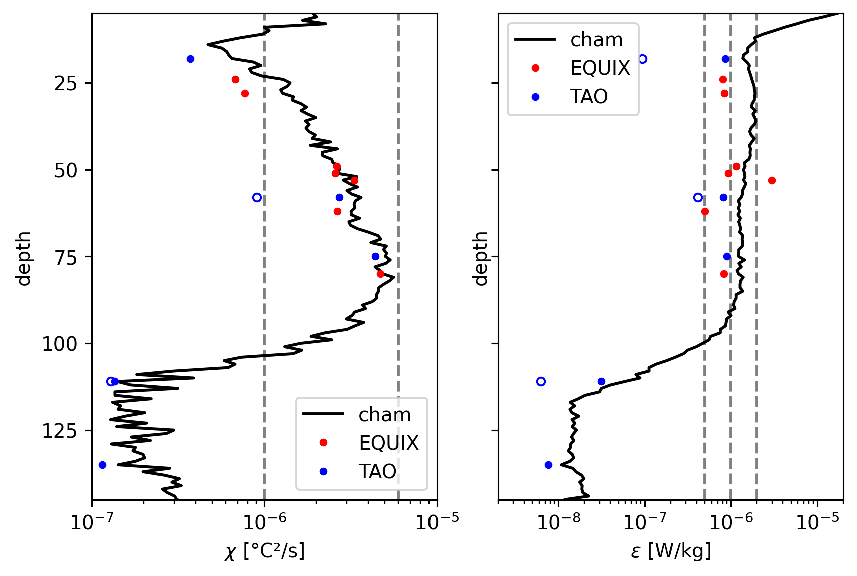
Conclusion: I can reasonably reproduce these figures, the differences are likely that in masking (I think I have a masked product). The only point of concern is that the TAO χpods are all systematically low by a factor of 2. I recombined these datasets from scratch, so it would be good to double-check that.
χ, ε#
Reproducing Perlin & Moum
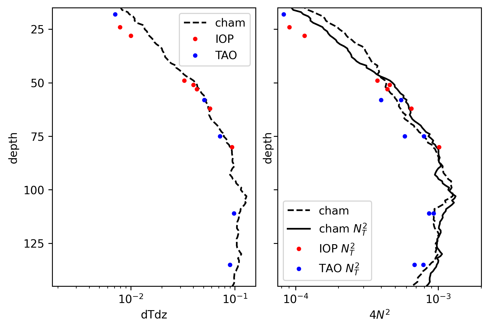
75m TAO ε is low
ε below 120m is higher than Perlin & Moum by quite a bit but χ compares well.
f, axx = plt.subplots(1, 2, sharey=True, constrained_layout=True)
ax = dict(zip(["chi", "eps"], axx))

for var in ax:
    cham[var].where(cham[var] < 1e-3).mean("time").cf.plot(
        xscale="log", color="k", ax=ax[var], label="cham"
    )
    iop[var].mean("time").cf.plot(
        marker=".", ls="none", label="EQUIX", color="r", ax=ax[var]
    )
    tao_iop[var + "1"].mean("time").cf.plot(
        marker=".", color="b", ls="none", label="TAO", ax=ax[var]
    )
    # iop[var + "2"].mean("time").cf.plot(marker=".", ls="none", label="IOP", color='r', ax=ax[var])
    ax[var].legend()
    tao_iop[var + "2"].mean("time").cf.plot(
        marker="o",
        markerfacecolor="none",
        ms=4,
        color="b",
        ls="none",
        label="TAO",
        ax=ax[var],
    )

ax["chi"].set_xlim([1e-7, 1e-5])
ax["chi"].set_ylim([145, 5])
ax["chi"].set_yticks([125, 100, 75, 50, 25])
dcpy.plots.linex([1e-6, 6e-6], ax=ax["chi"])

ax["eps"].set_xlim([2e-9, 2e-5])
dcpy.plots.linex([5e-7, 1e-6, 2e-6], ax=ax["eps"])
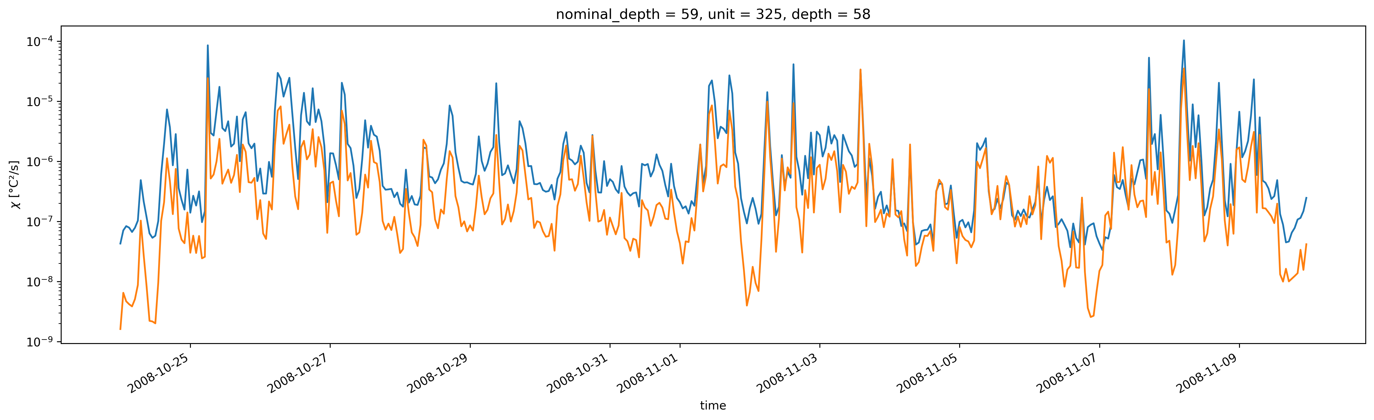
59m χpod sensor 2 is low, does not match Perlin & Moum.
tao_iop.chi1.sel(depth=58).plot(size=5, aspect=4)
tao_iop.chi2.sel(depth=58).plot(yscale="log")
[<matplotlib.lines.Line2D at 0x7fdcb8ee7a60>]
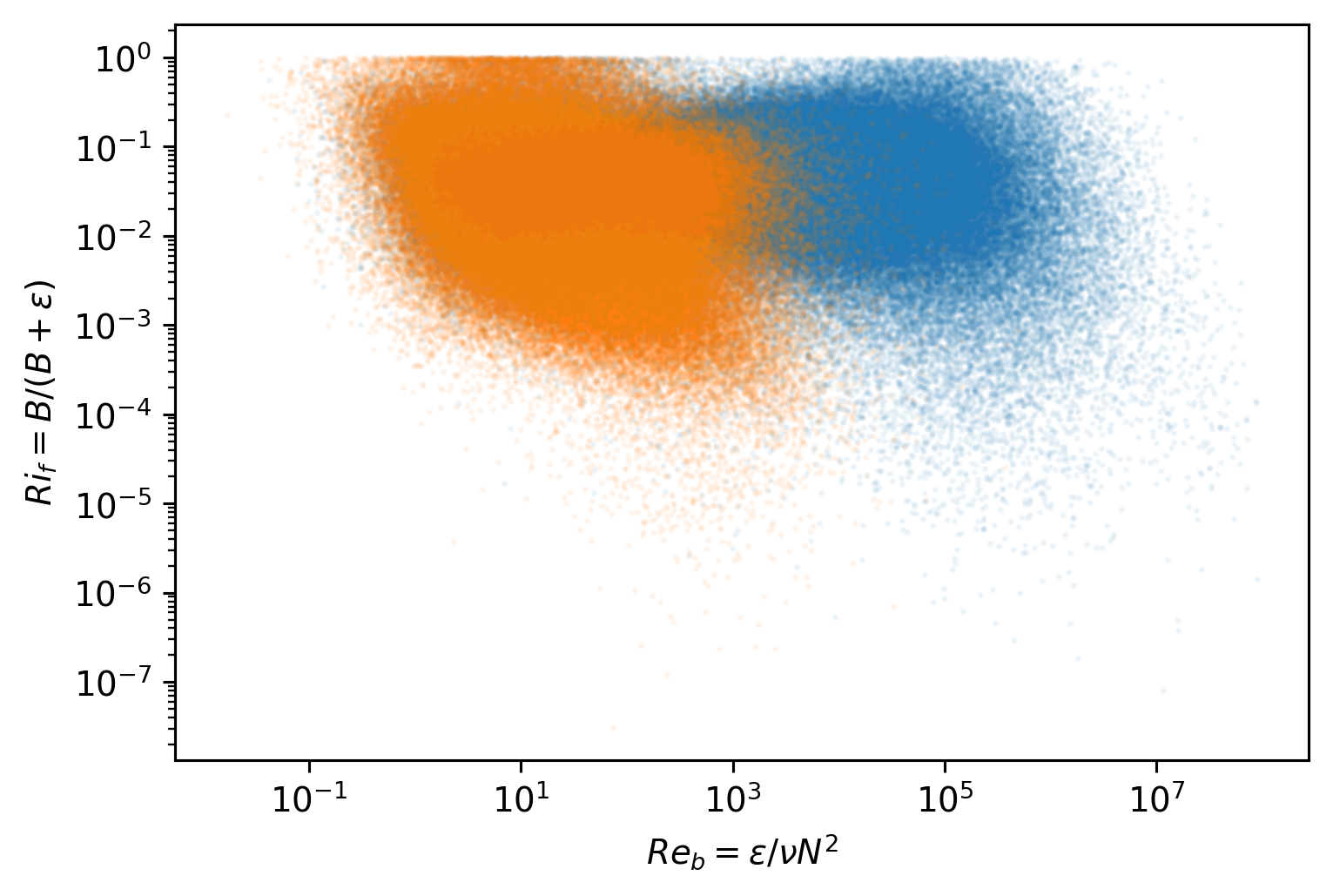
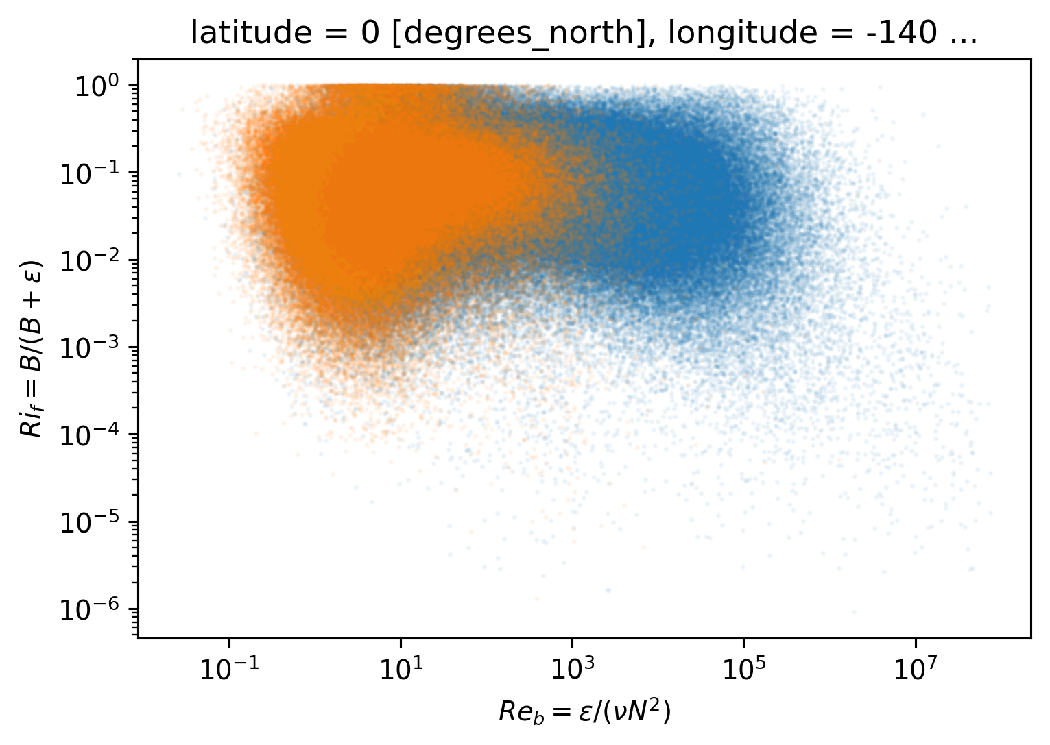
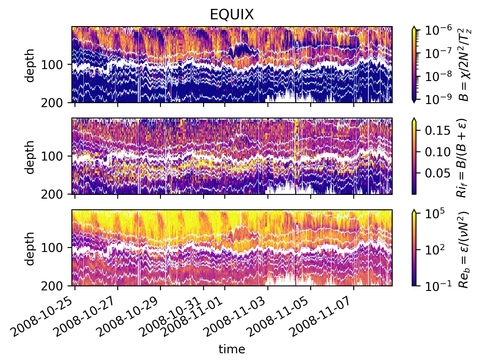
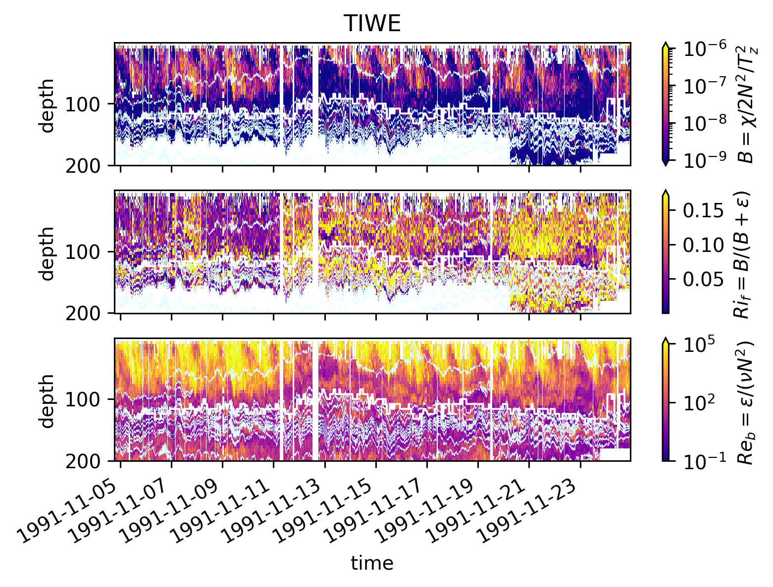
Variations in \(Ri_f\), \(Γ\)#
Γ is potentially a large uncertainty in \(J_q^ε\). Lets try the analysis of Monismith et al (2016). Definitions:
\begin{align*} Ri_f &= \frac{B}{B + ε} \ Re_b &= \frac{ε}{νN^2} \ B &= \frac{χ}{2} \frac{N^2}{T_z^2} \ Γ &= \frac{Ri_f}{1 - Ri_f} \end{align*}
I’m calculating gradients after thorpe-sorting by ρ
I’ll look at EQUIX and TIWE.
equixρ = chamρ
equixρ.attrs["name"] = "EQUIX"
tiweρ.attrs["name"] = "TIWE"
pump.calc.add_mixing_diagnostics(equixρ)
pump.calc.add_mixing_diagnostics(tiweρ)
Simple \(Re_b\) vs \(Ri_f\) scatter plot suggest two parameter regimes. More clearly in EQUIX
figs = tuple(
    np.log10(ds[["Reb", "Rif"]]).hvplot.hexbin(
        x="Reb",
        y="Rif",
        by=["depth", "time"],
        cnorm="eq_hist",
        logz=True,
        cmap="fire_r",
        title=ds.attrs["name"],
        frame_width=300,
    )
    for ds in [equixρ, tiweρ]
)

figs[0] + figs[1]
chamρ.where(chamρ.depth < chamρ.eucmax).plot.scatter(y="Rif", x="Reb", s=1, alpha=0.05)
chamρ.where(chamρ.depth > chamρ.eucmax).plot.scatter(y="Rif", x="Reb", s=1, alpha=0.05)
plt.gca().set_xscale("log")
plt.gca().set_yscale("log")
tiweρ.where(tiweρ.depth < tiweρ.eucmax).plot.scatter(y="Rif", x="Reb", s=1, alpha=0.05)
tiweρ.where(tiweρ.depth > tiweρ.eucmax).plot.scatter(y="Rif", x="Reb", s=1, alpha=0.05)
plt.gca().set_xscale("log")
plt.gca().set_yscale("log")
\(Ri_f\) : TIWE vs EQUIX#
Lets split the datasets into two: above, below the EUC (add 5m to EUC max depth as buffer).
These are contours of counts in logarithmically spaced bins, normalized by the maximum and plotted in log-log space.
The lines are means in coarser \(Re_b\) bins.
So I think this is a correct view of the dataset.
It appears the mean \(Ri_f < 0.17\) nearly always! Except at low \(Re_b\)
EQUIX: ~ 0.07
TIWE: ~ 0.11
f, ax = plt.subplots(1, 2, sharex=True, sharey=True, constrained_layout=True)
pump.plot.plot_reb_rif(equixρ, ax=ax[0])
pump.plot.plot_reb_rif(tiweρ, ax=ax[1])
f.set_size_inches((6, 3.5))
dcpy.plots.clean_axes(ax)
equixρ.mean_Rif
<xarray.DataArray 'mean_Rif' (euc_bin: 2, Reb_bins_2: 10)>
array([[0.18618021, 0.1075182 , 0.07767015, 0.07476665, 0.0756329 ,
        0.07256418, 0.07379563, 0.07677696, 0.07909978, 0.08519817],
       [0.21628219, 0.1277962 , 0.08692343, 0.06169491, 0.04539081,
        0.03710017, 0.0336863 , 0.03146146, 0.02810299, 0.02923173]])
Coordinates:
  * euc_bin     (euc_bin) <U5 'above' 'below'
  * Reb_bins_2  (Reb_bins_2) object (0.1, 0.3981071705534972] ... (25118.8643...
Attributes:
    long_name:      $Ri_f = B/(B+ε)$
standard_name: flux_richardson_numbertiweρ.mean_Rif
<xarray.DataArray 'mean_Rif' (euc_bin: 2, Reb_bins_2: 10)>
array([[0.09048535, 0.08779893, 0.10000951, 0.12460097, 0.12698226,
        0.12097309, 0.11412452, 0.10305291, 0.09247974, 0.0938887 ],
       [0.12942589, 0.10535563, 0.11015094, 0.13816754, 0.14245744,
        0.11932936, 0.10287794, 0.08853348, 0.07475338, 0.0822512 ]])
Coordinates:
  * euc_bin     (euc_bin) <U5 'above' 'below'
    latitude    int64 0
    longitude   int64 -140
  * Reb_bins_2  (Reb_bins_2) object (0.1, 0.3981071705534972] ... (25118.8643...
Attributes:
    long_name:      $Ri_f = B/(B+ε)$
standard_name: flux_richardson_numberTIWE#
tiwe["Jq_ε"] = (
    1025
    * 4000
    * 0.2
    * tiwe.eps.where(tiwe.eps < 1e-5)
    / tiwe.N2.where(tiwe.N2 > 1e-6)
    * tiwe.dTdz.where(tiwe.dTdz > 1e-4)
)
tiwe["Jq_χ"] = (
    1025
    * 4000
    * tiwe.chi.where(tiwe.eps < 1e-5)
    / 2
    / tiwe.dTdz.where(np.abs(tiwe.sortT.diff("depth")) > 1e-3)
)

tiwe.Jq.sel(depth=slice(11, None)).mean("time").cf.plot(y="depth")
tiwe.Jq_ε.mean("time").cf.plot(y="depth")
tiwe.Jq_χ.mean("time").cf.plot(
    y="depth", yincrease=False, xscale="linear", xlim=(0, 120), ylim=(200, 0)
)
[<matplotlib.lines.Line2D at 0x7faa0e310190>]
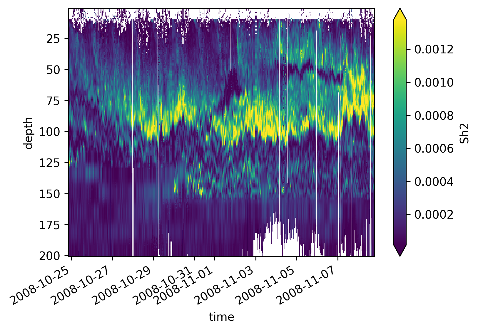
pump.plot.plot_mixing_diagnostics_timeseries(equixρ)
pump.plot.plot_mixing_diagnostics_timeseries(tiweρ)
equixρ.Sh2.cf.plot(x="time", robust=True)
<matplotlib.collections.QuadMesh at 0x7f873fbb0a90>
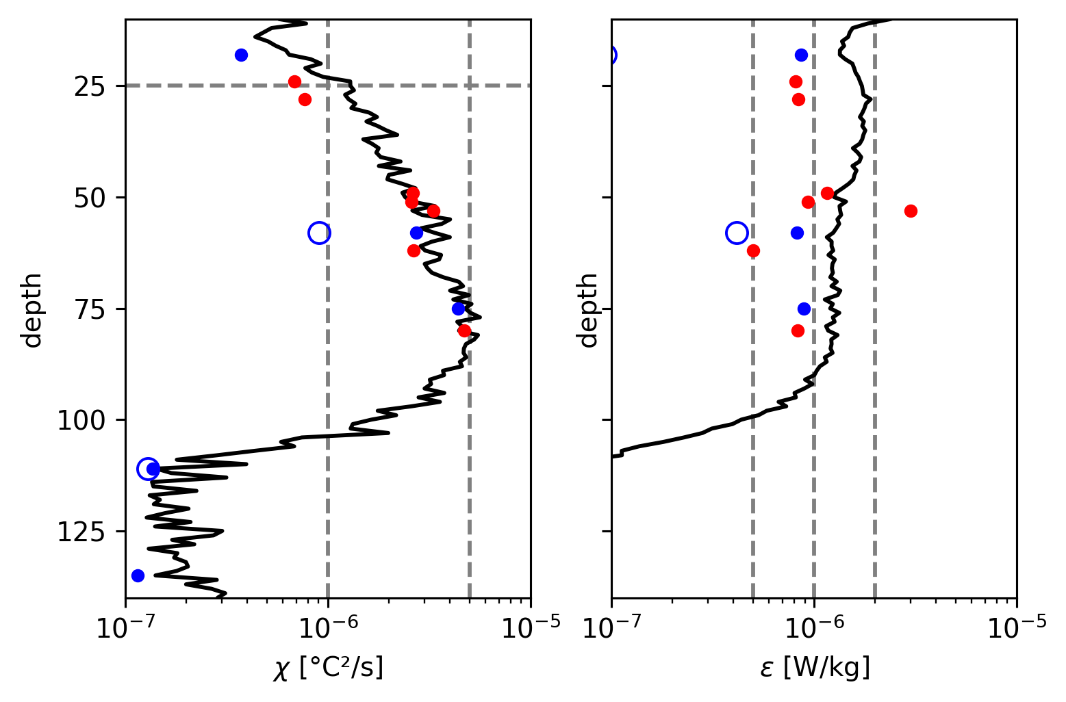
Reproducing Perlin & Moum (2012)#
I’m tuning max allowable χ, ε to visually match Perlin & Moum
Deepest 2 TAO χpods seem to be at wrong depths
TAO at 18m, 75m is too low.
~Need to save both sensors separately. If I did average then that’s an issue here.~ I did not average, just followed the comment and always picked sensor 1.
TODO:
Find all other sensor 2 data for EQUIX.
See if I can find Sasha’s merged files
f, ax = plt.subplots(1, 2, sharey=True)

for axx, var in zip(ax.flat, ["chi", "eps"]):
    cham[var].where((cham.chi < 1e-2) & (cham.eps < 6e-5)).mean("time").cf.plot(
        xscale="log", xlim=(1e-7, 1e-5), ylim=(140, 10), color="k", ax=axx
    )
    iop[var].mean("time").plot(
        y="depth", marker=".", color="r", ls="none", ms=8, ax=axx
    )
    tao_iop[var].mean("time").plot(
        y="depth", marker=".", color="b", ls="none", ms=8, ax=axx
    )
    tao_iop[var + "2"].mean("time").plot(
        y="depth", marker="o", color="b", ls="none", ms=8, ax=axx, fillstyle="none"
    )


ax[0].set_yticks([25, 50, 75, 100, 125])
dcpy.plots.liney(25, ax=ax[0])
dcpy.plots.linex([1e-6, 5e-6], ax=ax[0])
dcpy.plots.linex([5e-7, 1e-6, 2e-6], ax=ax[1])
Tz, N2#
f, axx = plt.subplots(1, 2, sharey=True, constrained_layout=True)
ax = dict(zip(["dTdz", "N2"], axx))

for var in ax:
    if var == "dTdz":
        (-1 * cham[var]).mean("time").cf.plot(
            ls="--", xscale="log", color="k", ax=ax[var], label="cham"
        )
    if var == "N2":
        (4 * cham["N2"]).mean("time").cf.plot(
            ls="--", xscale="log", color="k", ax=ax[var], label="cham"
        )
    if var != "N2":
        iop[var].mean("time").cf.plot(
            marker=".", ls="none", label="IOP", color="r", ax=ax[var]
        )
        tao_iop[var].mean("time").cf.plot(
            marker=".", color="b", ls="none", label="TAO", ax=ax[var]
        )
    if var == "N2":
        (4 * cham["NT2"]).mean("time").cf.plot(
            ls="-", label="cham $N_T^2$", color="k", ax=ax[var]
        )
        (4 * iop["NT2"]).mean("time").cf.plot(
            marker=".", ls="none", label="IOP $N_T^2$", color="r", ax=ax[var]
        )
        (4 * tao_iop["NT21"]).mean("time").cf.plot(
            marker=".", color="b", ls="none", label="TAO $N_T^2$", ax=ax[var]
        )
        (4 * tao_iop["NT22"]).mean("time").cf.plot(
            marker=".", color="b", ls="none", ax=ax[var]
        )

    ax[var].legend()
ax["N2"].set_xlabel("$4N^2$")
ax["N2"].set_ylim([145, 15])
ax["dTdz"].set_yticks([125, 100, 75, 50, 25])
# ax["dTdz"].set_xlim([7.5e-4, 2e-3])
ax["N2"].set_xlim([7.5e-5, 2e-3])
(7.5e-05, 0.002)
Explorations#
cham5m = cham.copy(deep=True)
cham5m["dTdz"] = cham5m.sortT.differentiate("depth")
# cham5m["dTdz"] = cham5m.theta.diff("depth")# / cham5m.depth.diff("depth")
# cham5m["dTdz"] = cham5m.dTdz.where(np.abs(cham5m.dTdz) > 5e-3)
cham5m["N2"] = 9.81 / 1025 * cham5m.pden.differentiate("depth")
cham5m = cham5m.where((cham5m.N2 > 5e-6) & (np.abs(cham5m.dTdz) > 1e-3))
# cham5m["N2"] = np.abs(cham5m.N2.where(cham5m.N2 > 5e-6))
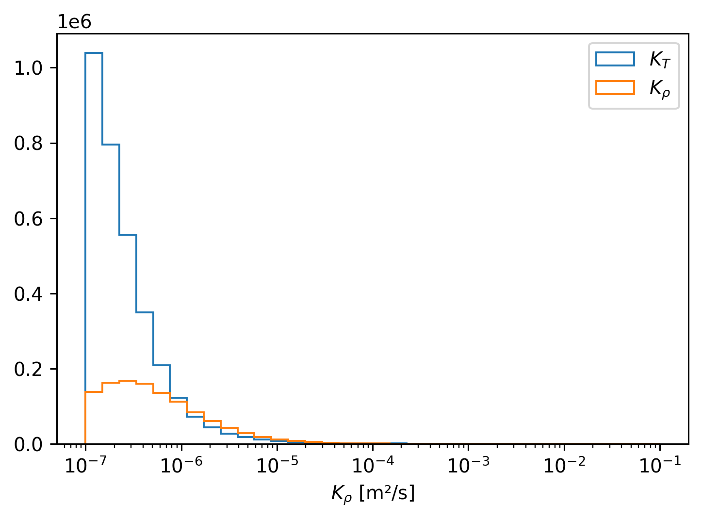
cham5m["KT"] = (
cham5m.chi / 2 / cham5m.dTdz**2
) # .where(np.abs(cham5m.dTdz) > 1e-3) ** 2
cham5m.KT.attrs = {"long_name": "$K_T$", "units": "m²/s"}
cham5m["Kρ"] = 0.2 * cham5m.eps / cham5m.N2
cham5m.Kρ.attrs = {"long_name": "$K_ρ$", "units": "m²/s"}
cham5m.chi.where(cham5m.chi < 1e-3)
cham5m["Jq_χ"] = 1025 * 4000 * cham5m.KT * cham5m.dTdz
cham5m.Jq_χ.attrs = {"long_name": "$J_q^χ$", "units": "W/m²"}
cham5m["Jq_ε"] = 1025 * 4000 * cham5m.Kρ * cham5m.dTdz
cham5m.Jq_ε.attrs = {"long_name": "$J_q^ε$", "units": "W/m²"}
cham5m.KT.plot.hist(
    bins=np.logspace(-7, -1, 35),
    xscale="log",
    histtype="step",
    density=True,
    label="$K_T$",
)
cham5m.Kρ.plot.hist(
    bins=np.logspace(-7, -1, 35),
    histtype="step",
    xscale="log",
    density=True,
    label="$K_ρ$",
)
plt.legend()
<matplotlib.legend.Legend at 0x7faa0b1a6a60>
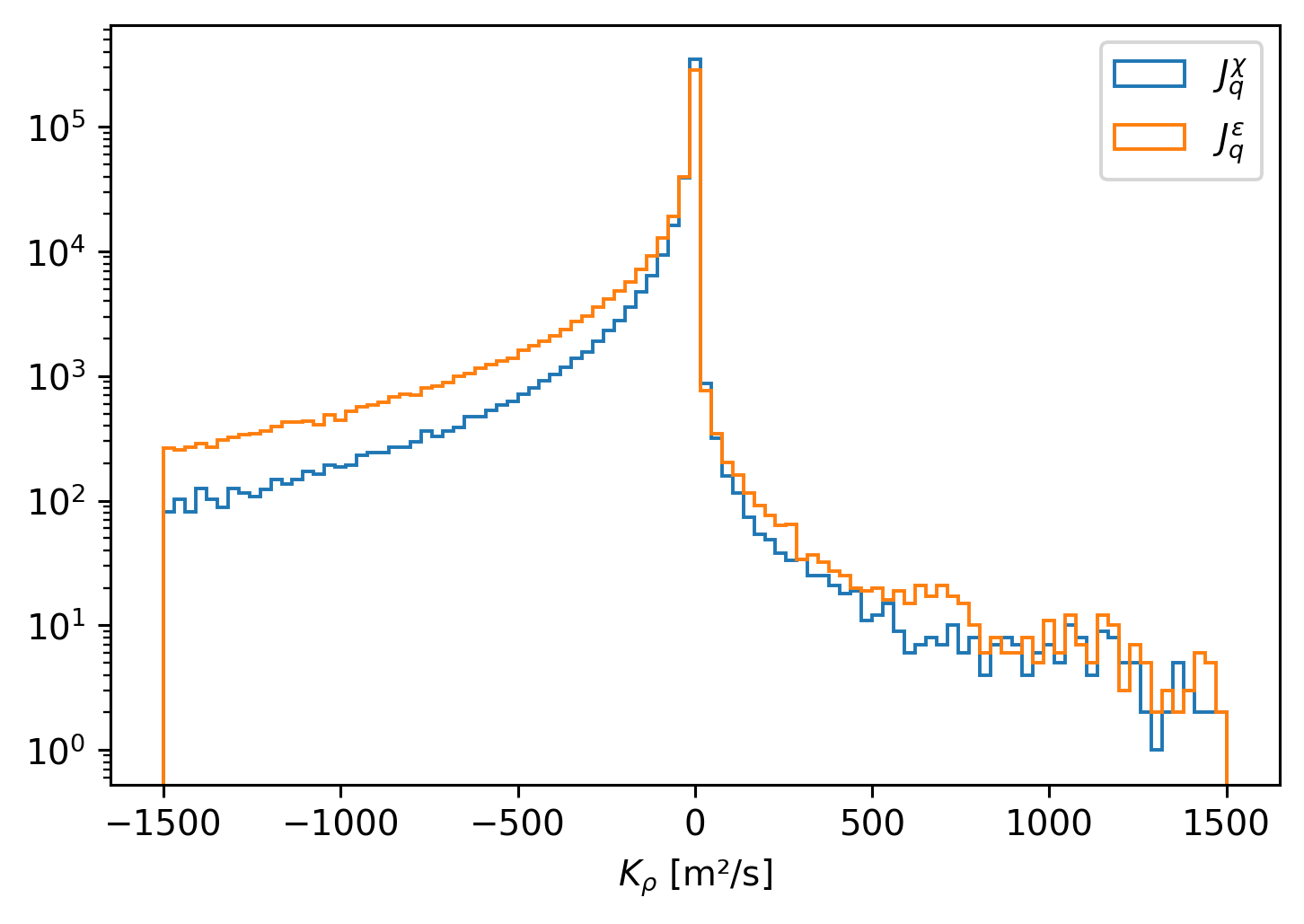
(4e6 * cham5m.KT * cham5m.dTdz).plot.hist(
    yscale="log", bins=np.linspace(-1500, 1500, 100), histtype="step", label="$J_q^χ$"
)
(4e6 * cham5m.Kρ * cham5m.dTdz).plot.hist(
    yscale="log", bins=np.linspace(-1500, 1500, 100), histtype="step", label="$J_q^ε$"
)
plt.legend()
<matplotlib.legend.Legend at 0x7fa9f6383670>
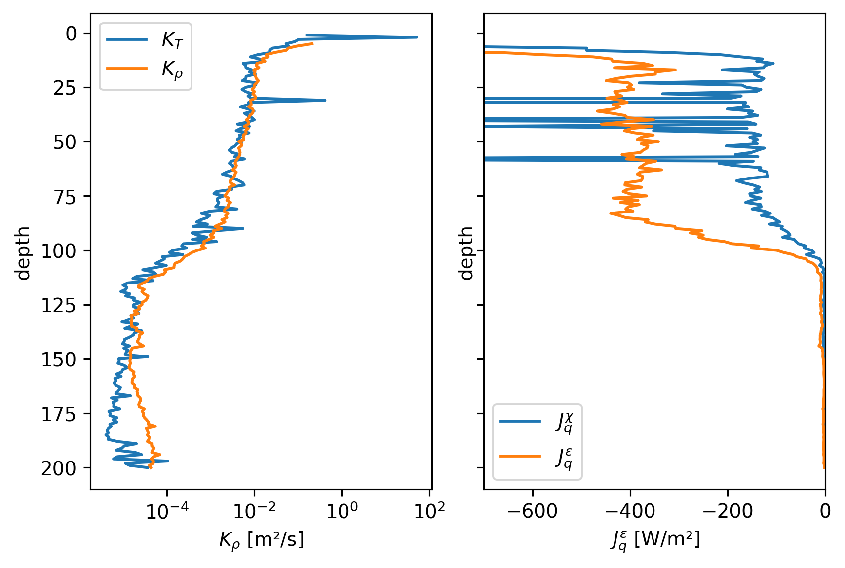
f, axx = plt.subplots(1, 2, sharey=True, constrained_layout=True)

cham5m.KT.mean("time").cf.plot(ax=axx[0], label="$K_T$")
cham5m.Kρ.mean("time").cf.plot(xscale="log", ax=axx[0], label="$K_ρ$")

cham5m.Jq_χ.where(cham5m.dTdz < 0).mean("time").cf.plot(ax=axx[1], label="$J_q^χ$")
cham5m.Jq_ε.where(cham5m.dTdz < 0).mean("time").cf.plot(
    xlim=(-700, 0), ax=axx[1], label="$J_q^ε$"
)

[ax.legend() for ax in axx.flat]
[<matplotlib.legend.Legend at 0x7fa9f814ab50>,
 <matplotlib.legend.Legend at 0x7fab86ba9340>]
Old Stuff#
Test thorpe sorting#
import pandas as pd

time = pd.Timestamp("2008-11-03 04:00:00")

profile = cham.sel(time=[time], method="nearest")
profile.theta.plot(hue="time")
thorpesort(profile.theta, profile.theta, ascending=False).plot(hue="time", marker=".")
thorpesort(profile.theta, profile.pden, ascending=True).plot(hue="time", marker="x")
[<matplotlib.lines.Line2D at 0x7fabc7d716a0>]
time = pd.Timestamp("2008-11-03 04:00:00")

theta_old.sel(time=time, method="nearest").plot()
theta_old.sel(time=time, method="nearest").plot(color="k", marker=".")
cham.theta.sel(time=time, method="nearest").plot(color="blue", marker="^")
cham.sortT.sel(time=time, method="nearest").plot()
cham.sortTbyT.sel(time=time, method="nearest").plot(color="r")
[<matplotlib.lines.Line2D at 0x7faba6b77640>]
Daily average flux profiles#
What is the time zone?
We need to know the base of the DCL. This is key to knowing where Jq ~ 0. This could be shallower than the EUC by ~40m or so.
Use χpod to decide where \(J_q → 0\)
Use \(Ri\) as in Smyth & Moum(2013) from ADCP + T
Where is the maximum convergence? What is the thickness? LES use \(Ri_g \approx 0.35\)
We would like an estimate of \(w_{ci}\) which means we need \(dJ/dz\).
Overarching question: How do we deploy χpods to get at the heat flux convergence?
Todo:
TAO \(Ri_g\) estimate + EQUIX ADCP \(Ri_g\) estimate to find DCL depth.
ΔJ_q from χpods; ΔJ_q from subsampled Chameleon
tao_iop.Jq.resample(time="D").mean()
<xarray.DataArray 'Jq' (depth: 5, time: 17)>
array([[7.06766784e+02, 1.01491038e+03, 1.84228211e+02, 1.06032515e+02,
        1.38550775e+02, 6.87792578e+01, 5.28428869e+01, 7.06474460e+01,
        2.10137107e+02, 6.69772591e+01, 2.60723861e+02, 1.57208380e+02,
        7.88250335e+01, 5.27598780e+01, 7.63957720e+01, 2.22939950e+02,
        8.94741025e+01],
       [3.71387404e+01, 2.59915060e+02, 3.49055526e+02, 1.62475940e+02,
        2.12025597e+02, 2.96243340e+02, 6.54940891e+01, 6.58761679e+01,
        6.62070213e+02, 2.23179245e+02, 1.54038479e+02, 1.13118956e+01,
        1.29795935e+01, 7.95744004e+00, 5.45438802e+01, 2.24527492e+02,
        1.04873125e+02],
       [1.55258627e-01, 1.22423027e+01, 2.00160614e+02, 1.35941349e+02,
        1.22637892e+02, 2.17440861e+02, 1.95103617e+02, 4.52559376e+01,
        5.23027138e+02, 1.78311757e+02, 3.25831480e+02, 2.78429747e+02,
        1.58383447e+01, 5.57895450e+01, 1.72105936e+01, 5.50925230e+02,
        1.03894163e+02],
       [1.97226244e+00, 1.29250576e+01, 6.93811813e+00, 1.14581072e+01,
        1.53190395e+01, 8.59733200e+00, 5.78671929e+00, 1.38474406e+01,
        8.03079889e+00, 2.60530496e+00, 2.94519797e+00, 7.50803939e+00,
        7.09364421e+00, 5.03990141e+00, 3.66806703e+01, 1.57767849e+00,
        1.05418158e+01],
       [4.05696314e-01, 2.10655363e+00, 3.74634020e-01, 3.35937952e+00,
        6.43241139e+00, 2.05689562e+01, 6.70650801e-01, 9.68049652e-01,
        2.05825292e+00, 3.85614970e-01, 8.33995402e-01, 2.86658934e-01,
        1.48935639e-01, 2.10514712e-01, 2.59076476e-01, 8.10937199e-01,
        8.64465736e-01]])
Coordinates:
  * time           (time) datetime64[ns] 2008-10-24 2008-10-25 ... 2008-11-09
    nominal_depth  (depth) int64 0 59 69 129 0
    unit           (depth) int64 313 325 319 327 321
* depth (depth) int64 18 58 75 111 135iop.Jq.resample(time="H").mean().plot(row="depth")
<xarray.plot.facetgrid.FacetGrid at 0x16af84b50>
tao = pump.obs.read_tao_zarr("ancillary").rename({"Ri": "Rig"})
/Users/dcherian/work/pump/pump/obs.py:545: RuntimeWarning: Failed to open Zarr store with consolidated metadata, falling back to try reading non-consolidated metadata. This is typically much slower for opening a dataset. To silence this warning, consider:
1. Consolidating metadata in this existing store with zarr.consolidate_metadata().
2. Explicitly setting consolidated=False, to avoid trying to read consolidate metadata, or
3. Explicitly setting consolidated=True, to raise an error in this case instead of falling back to try reading non-consolidated metadata.
  tao = xr.open_zarr("tao-gridded-ancillary.zarr", **kwargs)
---------------------------------------------------------------------------
KeyError                                  Traceback (most recent call last)
File ~/mambaforge/envs/pump/lib/python3.10/site-packages/xarray/backends/zarr.py:348, in ZarrStore.open_group(cls, store, mode, synchronizer, group, consolidated, consolidate_on_close, chunk_store, storage_options, append_dim, write_region, safe_chunks, stacklevel)
    347 try:
--> 348     zarr_group = zarr.open_consolidated(store, **open_kwargs)
    349 except KeyError:

File ~/mambaforge/envs/pump/lib/python3.10/site-packages/zarr/convenience.py:1187, in open_consolidated(store, metadata_key, mode, **kwargs)
   1186 # setup metadata store
-> 1187 meta_store = ConsolidatedMetadataStore(store, metadata_key=metadata_key)
   1189 # pass through

File ~/mambaforge/envs/pump/lib/python3.10/site-packages/zarr/storage.py:2644, in ConsolidatedMetadataStore.__init__(self, store, metadata_key)
   2643 # retrieve consolidated metadata
-> 2644 meta = json_loads(store[metadata_key])
   2646 # check format of consolidated metadata

File ~/mambaforge/envs/pump/lib/python3.10/site-packages/zarr/storage.py:895, in DirectoryStore.__getitem__(self, key)
    894 else:
--> 895     raise KeyError(key)

KeyError: '.zmetadata'

During handling of the above exception, another exception occurred:

GroupNotFoundError                        Traceback (most recent call last)
Input In [4], in <cell line: 1>()
----> 1 tao = pump.obs.read_tao_zarr("ancillary").rename({"Ri": "Rig"})

File ~/work/pump/pump/obs.py:545, in read_tao_zarr(kind, **kwargs)
    543     tao = xr.open_zarr("tao_eq_hr_gridded.zarr", **kwargs)
    544 elif kind == "ancillary":
--> 545     tao = xr.open_zarr("tao-gridded-ancillary.zarr", **kwargs)
    547 tao.depth.attrs.update({"axis": "Z", "positive": "up"})
    549 # tao = tao.chunk({"depth": -1, "time": 10000})
    550 # tao["densT"] = dcpy.eos.pden(35, tao.T, tao.depth)
    551 # tao.densT.attrs["long_name"] = "$ρ_T$"
   (...)
    554 # tao["dens"] = dcpy.eos.pden(tao.S, tao.T, tao.depth)
    555 # tao.densT.attrs["description"] = "density using T, S"

File ~/mambaforge/envs/pump/lib/python3.10/site-packages/xarray/backends/zarr.py:752, in open_zarr(store, group, synchronizer, chunks, decode_cf, mask_and_scale, decode_times, concat_characters, decode_coords, drop_variables, consolidated, overwrite_encoded_chunks, chunk_store, storage_options, decode_timedelta, use_cftime, **kwargs)
    739     raise TypeError(
    740         "open_zarr() got unexpected keyword arguments " + ",".join(kwargs.keys())
    741     )
    743 backend_kwargs = {
    744     "synchronizer": synchronizer,
    745     "consolidated": consolidated,
   (...)
    749     "stacklevel": 4,
    750 }
--> 752 ds = open_dataset(
    753     filename_or_obj=store,
    754     group=group,
    755     decode_cf=decode_cf,
    756     mask_and_scale=mask_and_scale,
    757     decode_times=decode_times,
    758     concat_characters=concat_characters,
    759     decode_coords=decode_coords,
    760     engine="zarr",
    761     chunks=chunks,
    762     drop_variables=drop_variables,
    763     backend_kwargs=backend_kwargs,
    764     decode_timedelta=decode_timedelta,
    765     use_cftime=use_cftime,
    766 )
    767 return ds

File ~/mambaforge/envs/pump/lib/python3.10/site-packages/xarray/backends/api.py:495, in open_dataset(filename_or_obj, engine, chunks, cache, decode_cf, mask_and_scale, decode_times, decode_timedelta, use_cftime, concat_characters, decode_coords, drop_variables, backend_kwargs, *args, **kwargs)
    483 decoders = _resolve_decoders_kwargs(
    484     decode_cf,
    485     open_backend_dataset_parameters=backend.open_dataset_parameters,
   (...)
    491     decode_coords=decode_coords,
    492 )
    494 overwrite_encoded_chunks = kwargs.pop("overwrite_encoded_chunks", None)
--> 495 backend_ds = backend.open_dataset(
    496     filename_or_obj,
    497     drop_variables=drop_variables,
    498     **decoders,
    499     **kwargs,
    500 )
    501 ds = _dataset_from_backend_dataset(
    502     backend_ds,
    503     filename_or_obj,
   (...)
    510     **kwargs,
    511 )
    512 return ds

File ~/mambaforge/envs/pump/lib/python3.10/site-packages/xarray/backends/zarr.py:800, in ZarrBackendEntrypoint.open_dataset(self, filename_or_obj, mask_and_scale, decode_times, concat_characters, decode_coords, drop_variables, use_cftime, decode_timedelta, group, mode, synchronizer, consolidated, chunk_store, storage_options, stacklevel)
    780 def open_dataset(
    781     self,
    782     filename_or_obj,
   (...)
    796     stacklevel=3,
    797 ):
    799     filename_or_obj = _normalize_path(filename_or_obj)
--> 800     store = ZarrStore.open_group(
    801         filename_or_obj,
    802         group=group,
    803         mode=mode,
    804         synchronizer=synchronizer,
    805         consolidated=consolidated,
    806         consolidate_on_close=False,
    807         chunk_store=chunk_store,
    808         storage_options=storage_options,
    809         stacklevel=stacklevel + 1,
    810     )
    812     store_entrypoint = StoreBackendEntrypoint()
    813     with close_on_error(store):

File ~/mambaforge/envs/pump/lib/python3.10/site-packages/xarray/backends/zarr.py:365, in ZarrStore.open_group(cls, store, mode, synchronizer, group, consolidated, consolidate_on_close, chunk_store, storage_options, append_dim, write_region, safe_chunks, stacklevel)
    349     except KeyError:
    350         warnings.warn(
    351             "Failed to open Zarr store with consolidated metadata, "
    352             "falling back to try reading non-consolidated metadata. "
   (...)
    363             stacklevel=stacklevel,
    364         )
--> 365         zarr_group = zarr.open_group(store, **open_kwargs)
    366 elif consolidated:
    367     # TODO: an option to pass the metadata_key keyword
    368     zarr_group = zarr.open_consolidated(store, **open_kwargs)

File ~/mambaforge/envs/pump/lib/python3.10/site-packages/zarr/hierarchy.py:1182, in open_group(store, mode, cache_attrs, synchronizer, path, chunk_store, storage_options)
   1180         if contains_array(store, path=path):
   1181             raise ContainsArrayError(path)
-> 1182         raise GroupNotFoundError(path)
   1184 elif mode == 'w':
   1185     init_group(store, overwrite=True, path=path, chunk_store=chunk_store)

GroupNotFoundError: group not found at path ''
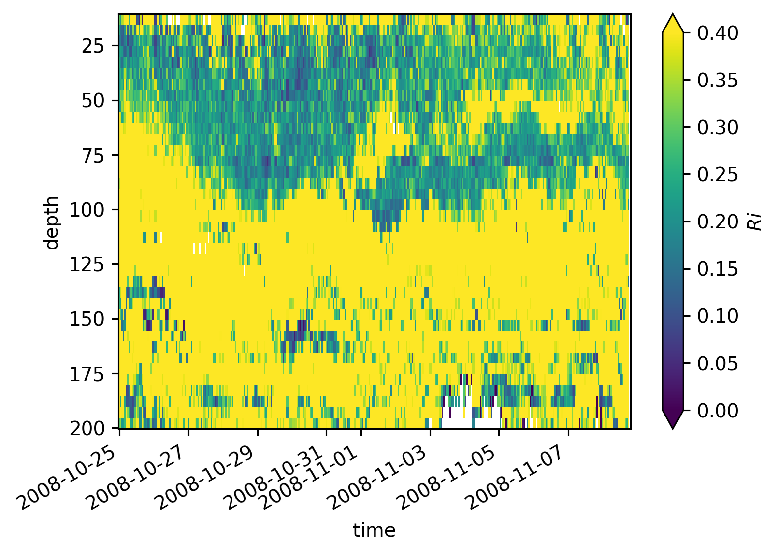
equix.Ri.cf.plot(robust=True, vmin=0, vmax=0.4)
<matplotlib.collections.QuadMesh at 0x169c8a020>
equix = pump.micro.make_clean_dataset(cham).sel(
    depth=slice(10, None), time=slice("2008-10-25", None)
)
/Users/dcherian/work/python/flox/flox/aggregate_flox.py:103: RuntimeWarning: invalid value encountered in true_divide
  out /= nanlen(group_idx, array, size=size, axis=axis, fill_value=0)
/Users/dcherian/work/python/flox/flox/aggregate_flox.py:103: RuntimeWarning: invalid value encountered in true_divide
  out /= nanlen(group_idx, array, size=size, axis=axis, fill_value=0)
/Users/dcherian/mambaforge/envs/pump/lib/python3.10/site-packages/xarray/core/nputils.py:169: RankWarning: Polyfit may be poorly conditioned
  warn_on_deficient_rank(rank, x.shape[1])
/Users/dcherian/mambaforge/envs/pump/lib/python3.10/site-packages/xarray/core/nputils.py:169: RankWarning: Polyfit may be poorly conditioned
  warn_on_deficient_rank(rank, x.shape[1])
/Users/dcherian/mambaforge/envs/pump/lib/python3.10/site-packages/xarray/core/nputils.py:169: RankWarning: Polyfit may be poorly conditioned
  warn_on_deficient_rank(rank, x.shape[1])
/Users/dcherian/mambaforge/envs/pump/lib/python3.10/site-packages/xarray/core/nputils.py:169: RankWarning: Polyfit may be poorly conditioned
  warn_on_deficient_rank(rank, x.shape[1])
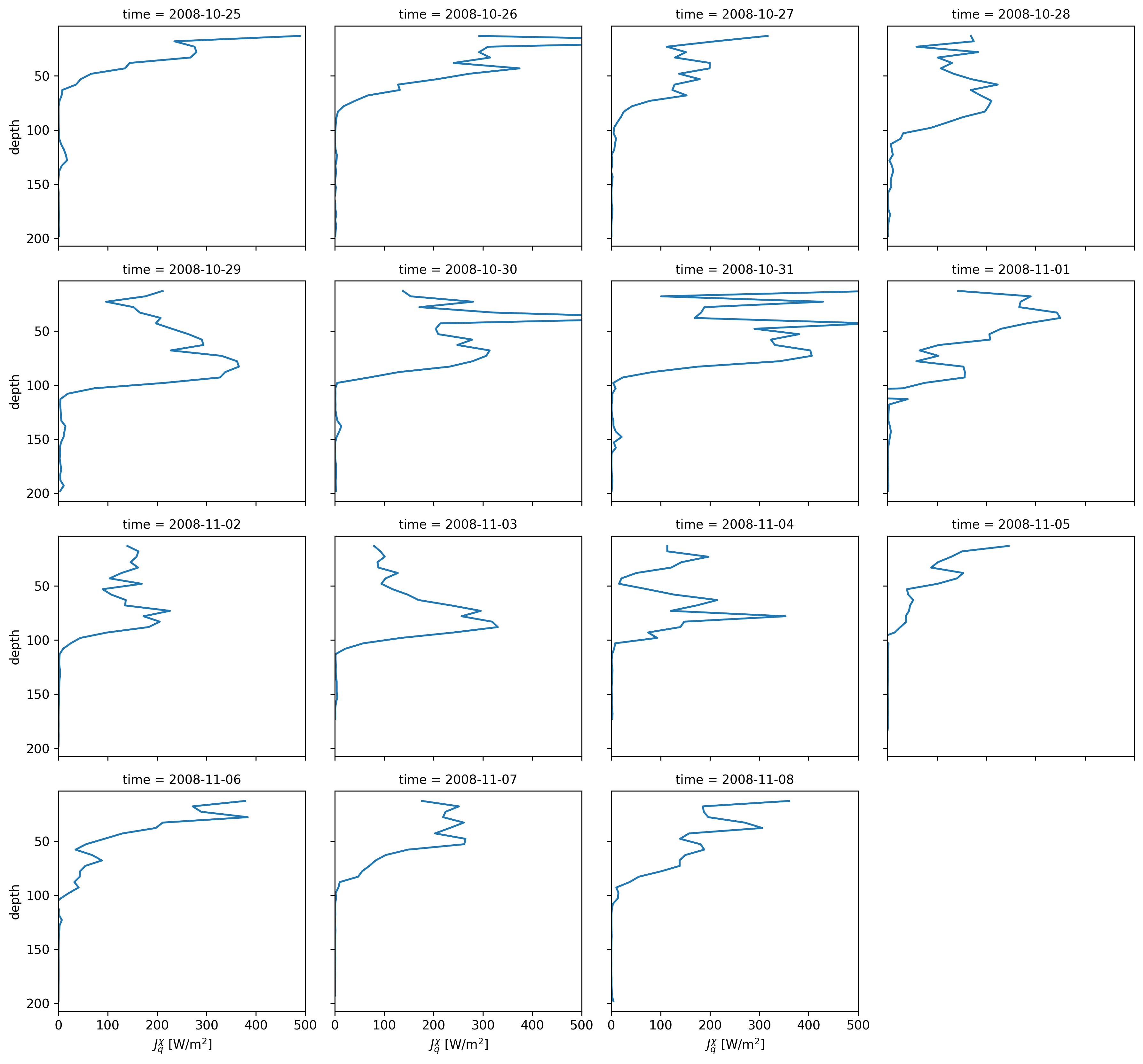
equix.Jq.resample(time="D").mean().cf.plot.line(col="time", col_wrap=4, xlim=(0, 500));
plt.rcParams["figure.dpi"] = 140
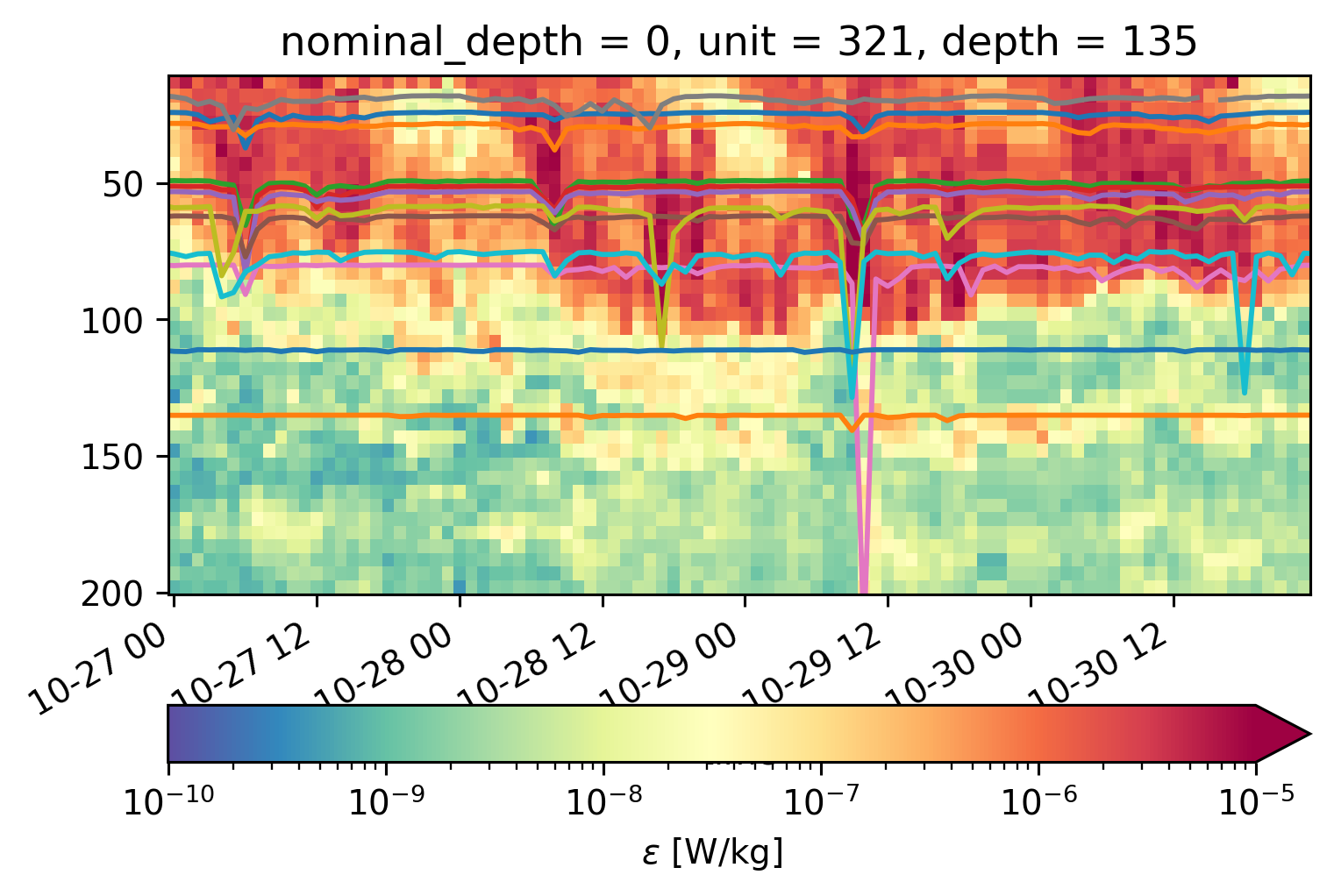
equix.eps.sel(time=slice("2008-10-27", "2008-10-30")).cf.plot(
    robust=True,
    norm=mpl.colors.LogNorm(1e-10, 1e-5),
    cmap=mpl.cm.Spectral_r,
    cbar_kwargs={"orientation": "horizontal"},
)

for z in iop.depth:
    j = iop.Jq.sel(depth=z)
    scaled = z + (j / 50)
    scaled.plot(x="time")


for z in tao_iop.depth:
    j = tao_iop.Jq.sel(depth=z)
    scaled = z + (j / 50)
    scaled.plot(x="time")
(
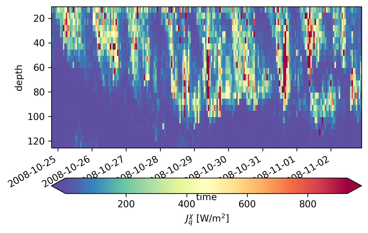
equix.Jq.sel(time=slice("2008-10-23", "2008-11-02"), depth=slice(125)).cf.plot(
robust=True,
cmap=mpl.cm.Spectral_r,
cbar_kwargs={"orientation": "horizontal"},
)
)
<matplotlib.collections.QuadMesh at 0x178715c00>
(
    j.sel(time=slice(None, "2008-11-10"))
    .groupby("time.day")
    .mean()
    .cf.plot.line(col="day", aspect=1)
)
<xarray.plot.facetgrid.FacetGrid at 0x1723dffa0>
